1  Introduction to NGS Sequencing

Next generation sequencing (NGS) revolutionised biology by providing rapid and cheap access to huge amounts of DNA sequence data. One unexpected benefit of the technology used in Illumina NGS sequencers was that it was also ideal for sequencing ultra-short ancient DNA.

In this chapter, we will go through:

• A brief overview of how DNA is structured
• How DNA sequencing works
• How most NGS sequenced DNA sequences are digitally represented

Finally we will cover some important considerations of NGS sequencing for ancient metagenomic datasets.

1.1 Basic Concepts

Basic structure of DNA

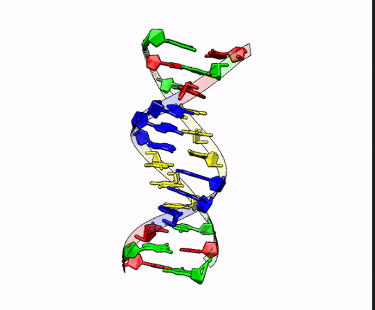
To understand how sequencing works, we first need to be familiar with the basic structure of DNA. Deoxyribonucleic acid (DNA) is present in the vast majority of cells in your body and is the biological molecule famous for it’s ‘double helix’ structure (Figure 1.1). It encodes all the genetic information required for the development, growth, and function of living organisms.

Each strand of the double helix structure consists of four main components called nucleotides, which bind together in different orders. These nucleotides can be grouped into two categories:

• Pyrimidines: cytosine (C) and thymine (T)
• Purines: guanine (G) and adenine (A)

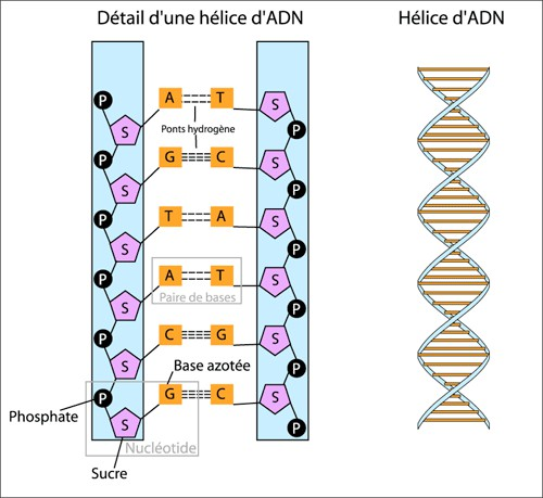
The nucleotides on one strand are connected via a sugar-phosphate ‘backbone’. The two strands are held together by the interaction of the hydrogen bond pairing between the four different nucleobases on each strand (Figure 1.2).

Figure 1.1: Still from an animation of a 3D model of the DNA double helix. Source: Erin Rod, CC BY 4.0, via Wikimedia Commons

Figure 1.2: 2D molecular diagram of a DNA helix, with the sugar-phosphate backbone and amine groups labelled indicated. Source: Pradana Aumars, CC BY-SA 4.0, via Wikimedia Commons

This pairing consists of one pyrimidine to one purine that are complementary to each other:

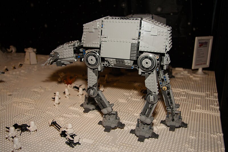
• C with G (to remember: think CGI in animated movies)
• A and T (to remember: think AT-AT Walker from Star Wars, Figure 1.3)

Therefore, whenever you find a C on one strand, you will normally find a G on the other strand (and vice versa), and the same for A and T.

What this means is that because of this complementary pairing, regardless of which strand you are ‘reading’, you can almost always reconstruct the order bases on the other strand.

Figure 1.3: Lego reconstruction of AT AT walker from Star Wars. Source: Tim Moreillon, CC BY-SA 2.0 Generic, via Wikimedia Commons

DNA replication

This complementary base pairing characteristic of a DNA molecule is a critical factor of how DNA gets replicated (or copied) within a cell.

At its core, DNA replication consists of:

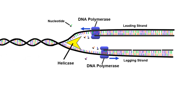
1. Unwinding the DNA helix and separating the two strands, by breaking the hydrogen bonds between the complementary bases using a helicase enzyme
2. Using a polymerase enzyme to add complementary new ‘free’ nucleotides floating in the cell to the exposed base on the strand (repeating this step for each base until a ‘stop’ signal is received)
3. Constructing bonds on the sugar-phosphate backbone of the new strand using a ligase enzyme

A graphical representation can be seen of a helicase enzyme separating strangds canbe seen in Figure 1.4.

Figure 1.4: Schematic diagram of DNA replication. A helicase unwinds DNA strand with DNA polymerases on the ‘leading’ and ‘lagging’ strand incorporating free nucleotides. Source: Christine Imiller, CC BY-SA 4.0, via Wikimedia Commons

This concept is important because it is the basis of how DNA sequencing works. With this, we can reconstruct the sequence of a DNA molecule for analysis.

Extracting DNA

To understand why specifically NGS sequencing revolutionised the field of palaeogenomics, we need to briefly compare the differences between how we get modern and ancient DNA.

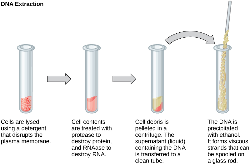
To get DNA from ‘modern’ samples (i.e., living organisms), first a biological tissue or sample is acquired. We then typically break down (lyse) the cell membrane and/or walls, to release the molecular contents of the cell (Danaeifar 2022). Extraction protocols then use a variety of enzymes or other mechanisms to degrade the other biomolecules in the cell (e.g., proteins, lipids, RNA) so that they do not ‘interfere’ with the extraction of the DNA itself. Finally, the DNA is separated and isolated out from the rest of the now-broken cell contents (purification).

This extracted ‘fresh’ DNA is typically in very long and intact strands that can be sort of imagined as long, soft spaghetti pasta like structures (Figure 1.5).

Figure 1.5: Simplified schematic diagram of the process of DNA extraction from living cells. Cell membranes are broken open, the extracted is treated to break down proteins and RNA, the DNA is separated out from the degraded biomolecules. Source: CNX OpenStax, CC BY 4.0 International, via Wikimedia Commons

In contrast, while the concept of ancient DNA extraction is very similar, the end product of the extraction is different.

Taking a skeleton as an example, once a bone has been sampled for bone podwer, cell lysis is normally not necessary as the cells are already broken down due to age. Instead, we have to ‘liberate’ the DNA from the mineral matrix of the bone. So palaeogenomicists first demineralise the bone to release the DNA, before degrading the remaining non-nucleic acid biomolecules in the sample (typically with proteinases) and then purifying the DNA (Andreeva et al. 2022).

In contrast, the resulting DNA molecules are quite different from the modern DNA. Rather than well cooked, soft spaghetti structures - ancient DNA molecules are more like extremely overcooked spaghetti. These molecules are highly degraded, broken down into very small fragments, and also often have ‘damage’ at the ends in the form of ‘modified nucleotides’ that do not represent the original sequence (Dabney, Meyer, and Pääbo 2013, and see the Introduction to Ancient DNA chapter for more information).
Finally, the small amount of tiny and damaged DNA molecules typically sits in a ‘soup’ of ‘contaminating’ high-quality modern DNA from the surrounding burial and storage environment (Figure 1.6).

As we will find out in the next section, these short fragments of DNA is not necessartily a disadvantage for NGS sequencing, but rather a benefit.

Figure 1.6: © Lucy Reading-Ikkanda for The Scientist Magazine, June 2015 (reused here with permission). Very small fragmented ‘endogenous’ DNA is preserved in bone, but alongside more recent and modern contaminating microbial and recent human DNA also present within and around the mineral matrix.

DNA sequencing

Now that we have our DNA, we want to be able to ‘read’ the order of the sequence of nucleotides that makes up a strand of the molecule.

Sequencing is the process of converting the long sequences of the four chemical nucleotides to the ACTG we can see on our computer screen. The result of this process is what we essentially apply all of our (meta)genomic analyses upon.

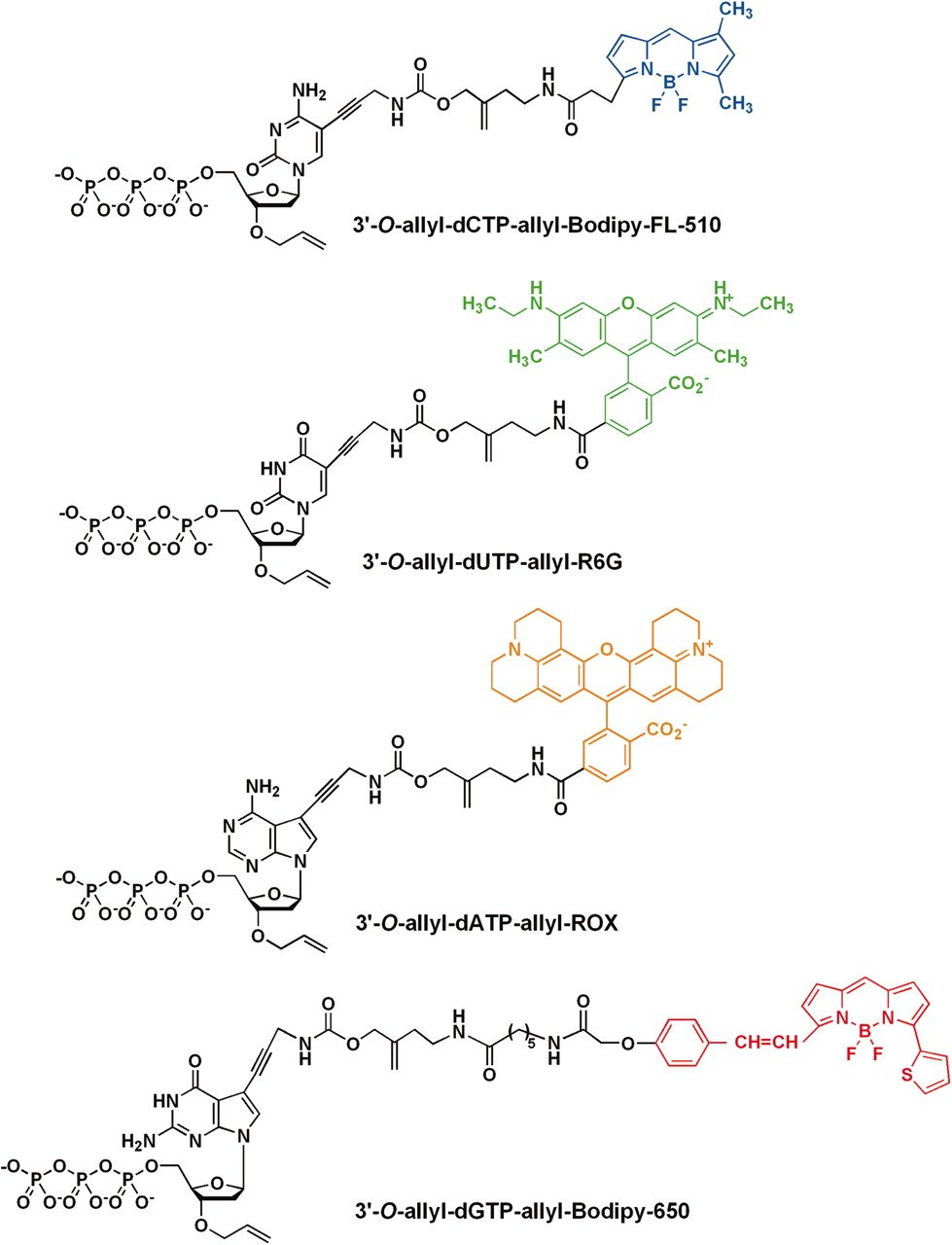
The core concept of most NGS sequencing methods ¹ is to replicate the strand as normal. But instead of adding a standard nucleotide, we instead incorporate a modified nucleotide with a fluorophore attached to it. A type of fluorophore is a small molecule that emits a specific colour when excited by a laser. As there are four different nucleotides, each will emit a different colour (Ju et al. 2006). Therefore if we record the colour emitted each time a modified nucleotide is added to a strand, we can reconstruct the sequence of the DNA nucleotides in order (Figure 1.7).

Figure 1.7: Molecular diagram of the four DNA nucleotides modified to include amine groups with fluorophores that will emit light when excited by a laser. Source: (Ju et al. 2006)

Sanger sequencing

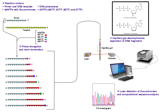
Historically, the first mass-production sequencing method was called Sanger sequencing (Figure 1.8) (Sanger, Nicklen, and Coulson 1977). This was the method used for sequencing the first human genome during the Human Genome Project (Heather and Chain 2015).

The concept of Sanger sequencing involves making many copies of a single DNA molecule using replication. However, when adding the free nucleotides, within the replication mixture of a pool of (normal) free nucleotides are a proportion of the modified nucleotides mentioned above. These modified nucleotides include the ability to that emit light when excited by exposure of certain wavelengths or give off specific radiation signatures (Valencia et al. 2013). In addition to the light emitting property, these modified nucleotides also contain a ‘blocking’ component that, once incorporated into the strand, prevents any further extension of the strand by other nucleotides.

Critically, as there is only a small proportion of blocking nucleotides amongst the pool of free nucleotides,the incorporation of the blocking nucleotides occurs at a slow rate and at different points during the replication process (J. A. Shendure et al. 2011). This results in many replicates of the original molecules but all at different lengths (Figure 1.8).

Figure 1.8: Diagram of sanger sequencing, with a primer, template and free blocking nucleotides being added to ends of molecules at random lengths. The molecules are passed through a size-selecting capillary with a light detector, which identifies which of the four blocking nucleotides are passing through the capillary at a given point and recorded in a chromatogram. Source: Estevezj, CC BY-SA 3.0 Unported via Wikimedia Commons

Once many different-length replicates of the template molecules are ready, the Sanger sequencing method involves running the pool of DNA fragments through a capillary gel. As all the molecules are of different sizes, they will move through the gel at different speeds, and therefore spread out based on the length of the molecule (Valencia et al. 2013). In modern sanger sequencing machines, a laser is fired at the gel at regular intervals, and the light emitted from the modified nucleotides is detected. Shorter molecules will move faster through the gel, and therefore will be detected first, whereas longer molecules will be detected later. Therefore, by detecting the light emitted as the incrementally longer molecules pass through the gel, we can reconstruct the sequence of the nucleotides along the module.

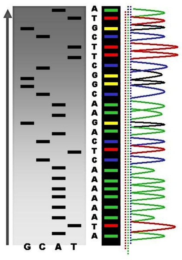
The result is a chromatogram, which is a graph that records the strength of each colour at each point in the gel band (Figure 1.9).

Figure 1.9: Example of a gel-based chromatogram with four columns with different bands. Each column corresponds to a different nucleotide and the light that is emitted at that position along the molecule. On the right is intensity graph of each colour given off by each modified nucleotide at each position. Source: Morse Phoque (Abizar), CC BY-SA 3.0 Unported via Wikimedia Commons

While this method was used for the first sequencing of the human genome, it was very slow and very expensive. It does not scale well due to the requirement of having many redundant copies to sequence each molecule (Schloss et al. 2020). Furthermore, this method also requires a large amount of starting DNA. This is problematic when we are handling degraded ancient DNA, as it is very rare to have a sufficient concentration of DNA to be able to use Sanger with sequencing - unless the initially preservation is high enough, and/or we take very large amounts input sample (which is typically via destructive methods).

1.2 Next generation sequencing

In 2005 the first ‘Next Generation Sequencing’ (NGS) machines were released ², in the form of Roche’s 454 Pyrosequencing (Heather and Chain 2015).

These new sequencers were able to quickly and cheaply sequence millions of DNA molecules at once, revolutionising genetics and enabling ‘accessible’ genomics to a much wider group of scientists (Koboldt et al. 2013).

While a few companies emerged with competing NGS sequencers employing different techniques, such as PacBio and IonTorrent, the platform that has been by far the most successful is the one from Illumina (Heather and Chain 2015). These Illumina machines have been so successful, they have almost exclusively sequenced the entire corpus of ancient DNA sequencing data. Therefore the rest of this chapter will focus just on Illumina sequencing.

Illumina sequencing

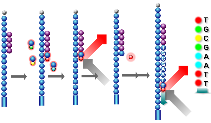
Illumina sequencing relies on a process termed ‘Sequencing by synthesis’ (SBS) but with reversible terminators (J. Shendure and Ji 2008). This follows a similar concept as Sanger Sequencing in that we add modified nucleotides with fluorophores for emitting per-nucleotide light. However instead of using multiple molecules of different lengths that are separated via a gel, it uses nucleotides that can be reversibly blocked, and thus after removing the ‘block’ can continue incorporating nucleotides within a single molecule (Bentley et al. 2008).

This works by immobilising the DNA so it stays at one location on a special type of plate (J. Shendure and Ji 2008). The machine then performs a typical DNA replication, adding fluorophore modified nucleotides one at a time. Instead of a chromatogram, the machine takes a type of photo of the emitted light. However the key difference is that when after this photo is taken, the blocking part of the oligo is removed, so the next modified oligo can added.

To visualise how this looks like, we can imagine looking down at a rectangular plate. On this surface, we can see millions of coloured tiny dots (Figure 1.10), that are all changing colour in realtime as each new nucleotide is added along the new strand.

Figure 1.10: Graphical representation of an Illumina sequencing flowcell during sequencing. Each colour dot corresponds to a single cluster of copies of the same DNA molecule emitting light corresponding to a single nucleotide along the molecular sequence.

However, before we start to capture the images of the new nucleotides on an Illumina platform, we need to prepare the DNA molecules in a specific way.

Flow cells and adapters

To ensure that DNA molecules do not move while recording the light being emitted by a modified nucleotide, in Illumina sequencing the DNA molecules are bound to a special glass slide called a flowcell (Figure 1.11). This also ensures the DNA does not get washed away during the sequencing process as different solutions wash through the machine between each step.

Figure 1.11: Schematic diagram of a Illumina HiSeq-like flowcell. The glass slide has eight ‘lanes’ (top), with wells at each end of each lane. The sequencing library is injected into the well, and moves through the lane in the direction as indicated by the arrows. Indicated by the dark green dots at the the bottom of each lane are the synthetic oligonucleotides that capture the DNA molecules, also known as the ‘lawn’. Image based on and inspired by Bronner et al. (2013) .

Figure 1.12: Photo of a lawn of grass, as a metaphor of the ‘lawn’ of artificial oligonucleotide sequences of an Illumina flowcell. Source: Animaldetector, CC BY-SA 3.0 via Wikimedia Commons

To immobilise the DNA, the flow cell is coated with a ‘lawn’ (Figure 1.12) of synthetic oligonucleotides (i.e., artificially produced DNA molecule with a specific and known sequence also known as ‘oligos’) (Holt and Jones 2008). By attaching (i.e., ligating) the complementary sequence of the synthetic oligos to the DNA molecules from our sample, when our DNA molecules flow over the lawn (Figure 1.11), the complementary bonds between the oligos on the lawn and the complementary sequence on our DNA molecules will form. This then will hold the DNA in place and ‘immoblise’ it for capturing emitted light at a specific location on the flow cell.

The process of adding the complementary synthetic oligos, referred to as ‘Adapters’, to the DNA molecules of a sample is called ‘Library preparation’.

These adapter sequences not only include the complementary sequence to flowcell oligos, but also an additional sequence that acts as a priming site for polymerases to start the replication process. Furthermore, researchers have exploited the ability of Illumina sequencers to sequence millions of molecules at once, to allow them to also sequence multiple samples at once. They do this by adding additional sequences to the adapter sequence construct that consist of short sample-specific ‘indices’ or ‘barcodes’ (Kircher, Sawyer, and Meyer 2012). These indices allow DNA molecules from different samples to be sequenced at the same time, and then separated back into the groups of molecules from the same samples during data analysis. This system of sequencing multiple samples at once is known as ‘multiplexing’ (Church and Kieffer-Higgins 1988).

Figure 1.13: Annotated library construct of a DNA molecule prepared for sequencing on Illumina platforms. The P5 and P7 primers are complementary to the flow cell oligo ‘lawn’, the i5 and i7 indices act as the library specific ‘barcode’ used for separating samples when performing multiplex-sequencing, The Read 1 and Read 2 primers act as priming sites for sequencing the template molecule (in this, case an ancient DNA molecule). Emojis from

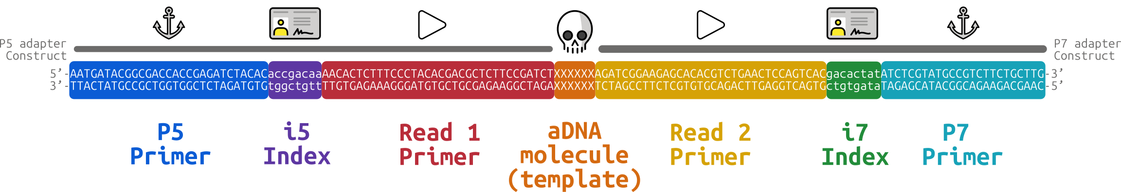
The completed index, adapter, and target DNA molecule construct (Figure 1.13) of all molecules from a given construction protocol run is termed a library, and this is what is injected into the sequencing machine.

Clustering

Once a library is injected into a flowcell, and each DNA molecule of the library is bound to it’s unique own location on the flowcell, we could start sequencing. However, there is the problem that the light emitted from a single tiny fluorophore is not strong enough to be captured by the camera in the sequencer.

The Illumina platforms get around this through a process called ‘clustering’ (Heather and Chain 2015). The clustering process makes many identical copies of the molecule right next to the original template molecule. When this cluster of DNA copies emit the light from the same nucleotide along their sequence at the same time, the light collectively emitted will now be sufficiently strong to be captured by the camera.

To make sufficient copies of the ‘template’ molecule efficiently, this clustering is carried out using ‘bridge amplification’ (Bentley et al. 2008).

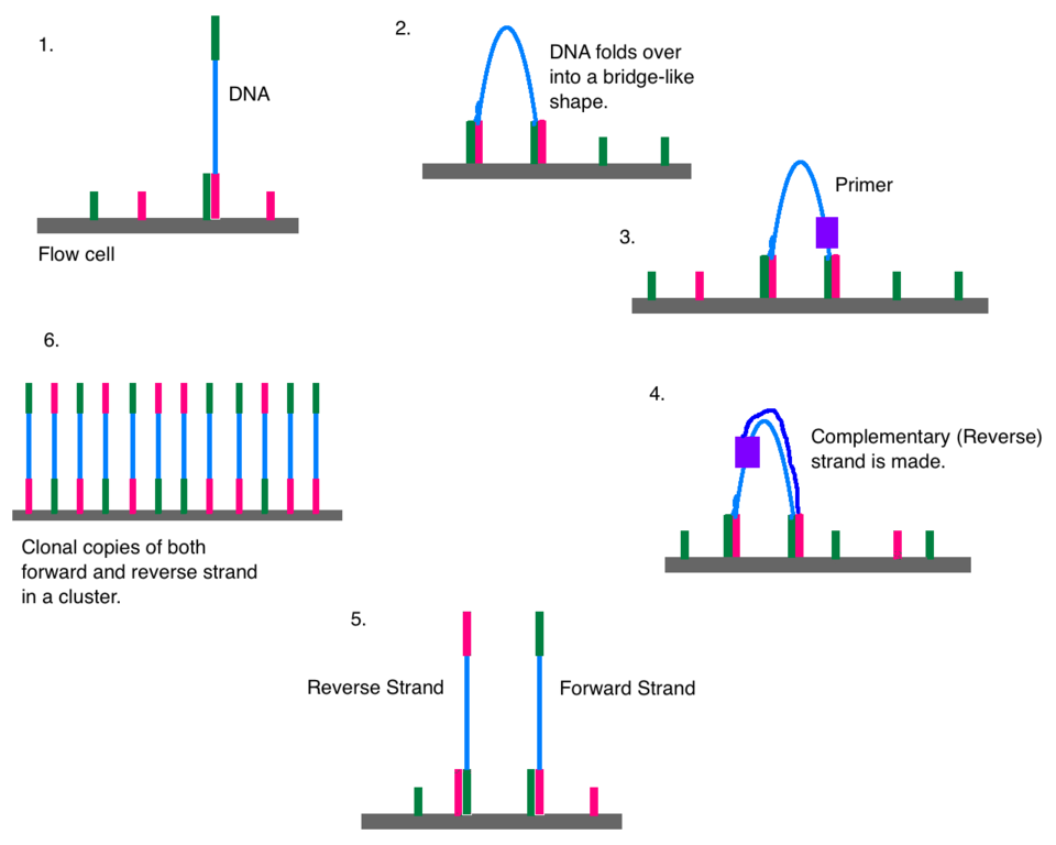
The process of bridge amplification is as follows:

1. A single-stranded DNA molecule is immobilised on the flow cell via the adapter at one end of the module
2. The DNA is ‘bent over’
3. The oligo adapter at the other end of the molecule binds to another complementary flow-cell oligo in its close vicinity (forming a bridge)
4. A priming sequence, free nucleotides, and a polymerase is then added to the flow cell
5. The reverse complement of the DNA molecule is made via replication, and the polymerase mixture is washed away
6. The two strands are then separated to form two single-stranded DNA molecules (with the new strand representing the reverse complement of the original template molecule)
7. Repeat 1-5 for the two new strands until sufficient copies are made

This process is also depicted in Figure 1.14.

Figure 1.14: Diagram of bridge amplification. Single stranded DNA molecules are bound to a flow cell using adapter sequences to complementary oligos on the flow cell. The molecule and chemically bent over so the reverse end also binds, and a polymerase reconstructs the complementary strand. The two strands are separated by cleaving of one adapter, representing the ‘forward’ and ‘reverse’ strand. Both strands undergo the same process repeatedly to make many copies. Source: DMLapato, CC BY-SA 4.0 International via Wikimedia Commons

Of course, after had many cycles of replication, we will have in a single cluster both forward and reverse complement copies of the same DNA molecule. As this would emit two different colours at each position along the sequence, one of the strand ‘directions are’ removed by ‘trimming’ the flow cell lawn at one of the adapter sequences

Sequencing-by-synthesis

With our cluster of many copies of the same DNA molecule all in the same direction, we can now start the ‘Sequencing by synthesis’ (SBS) process itself.

As with replication and Sanger sequencing, SBS involves adding free modified nucleotides to the template strand (with only the complementary base being able to be incorporated to the exposed strand at any one point), the modified nucleotides are excited with a laser, and a picture is taken (Bentley et al. 2008).

The main difference with Sanger sequencing is we can actually reuse the same DNA molecule to add more nucleotides along the same strand - rather than ‘discarding’ due to the permanently blocking nucleotides. This makes the SBS technique more resource sufficient, both in reagents (you need fewer copies of the molecule and recycle the same original copies of template molecules), but also in space as it is not necessary to separate out the molecules in a gel. Instead, they can be all fixed in a tightly packed layout on the flowcell.

Figure 1.15: Diagram of sequencing by synthesis. Free modified nucleotides bind to a strand next at a priming site. The blocking fluorophore prevents other nucleotides from binding, and when excited by a laser, emits a light specific to that nucleotide type the colour of which is recorded by a camera. The blocking fluorophore is cleaved off and the cycle repeats with the next nucleotide along the seqeuence. Source: Abizar Lakdawalla, CC BY-SA 3.0 Unported via Wikimedia Commons

The process as depicted in Figure 1.15 can be broken down to:

1. On a single stranded molecule, bind a primer to the molecule’s adapter priming site
2. Add fluorescently labelled nucleotides (with a reversible terminator) to the flow cell
3. Only complementary (modified) nucleotides will bind to the template strand at the first exposed base
4. Wash away unbound nucleotides
5. Fire a laser to excite the modified nucleotides to emit the corresponding colour, and take a picture
6. Clip off the fluorophore part of the nucleotide
7. Repeat 2-6 until the entire strand is sequenced

On Illumina sequencers, the number of repetitions (known as cycles) typically happens either 50, 75, or 150 times, depending on the machine and the type of sequencing chemistry kit.

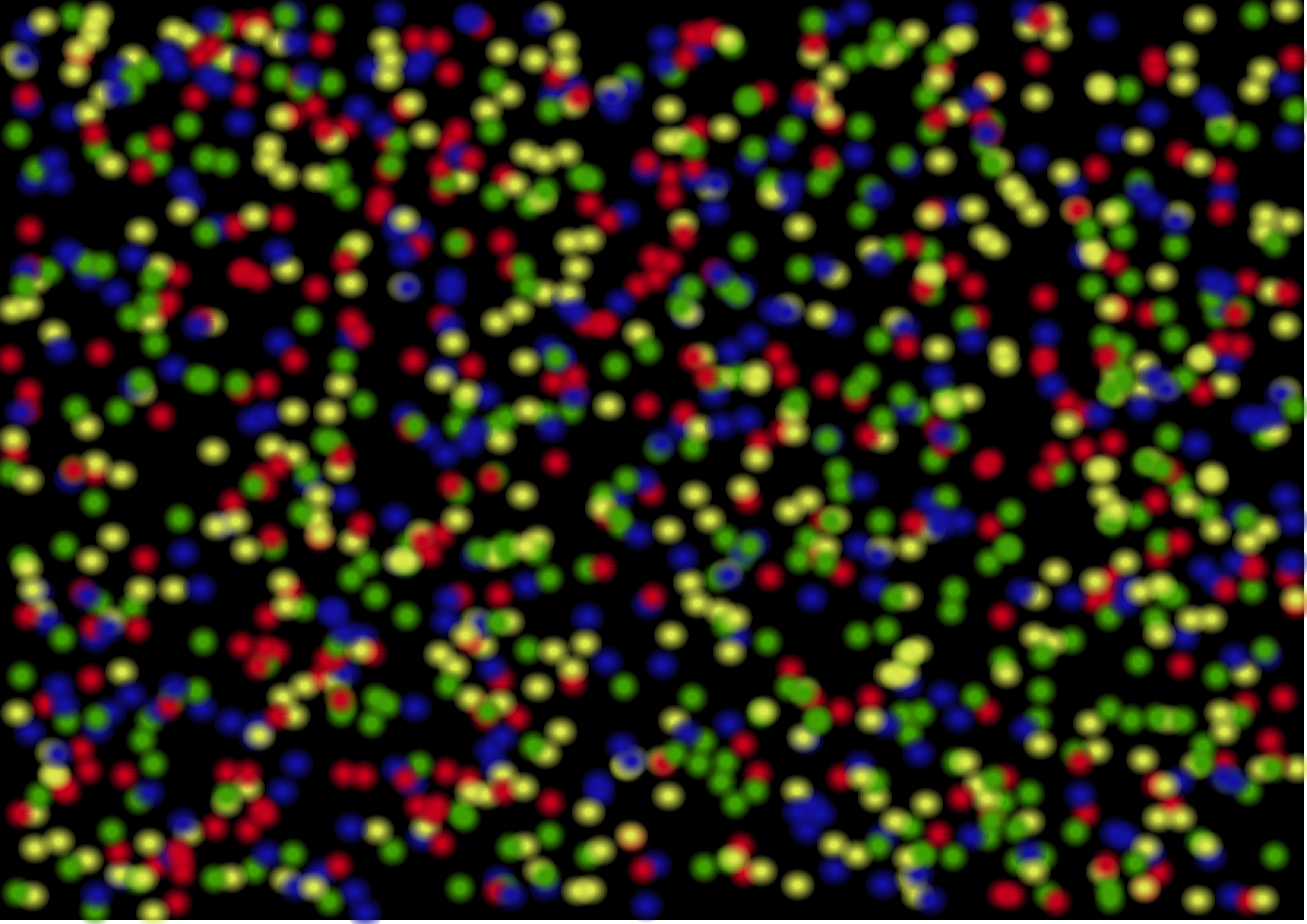
We can see a small fraction of such a flow cell in Figure 1.16. Each coloured dot corresponds to a cluster of DNA molecules. At each cycle (each photo), a new nucleotide is added to the strand, and a laser is fired to excite the fluorophores. We can see two different clusters emit different lights, as they are different DNA molecules and thus have different nucleotides at that particular ‘cycle’ (or position in the sequence) of the ‘replication’ process. By converting the emitted light to the known corresponding A, C, G, T, at each photo, we can reconstruct the sequence of the DNA molecule.

Figure 1.16: Diagram of sequencing by synthesis. Each frame represents a camera photo taken at the same location on the flow cell. Each coloured dot represents a different cluster of many copies of the same immoblised DNA molecule. By recording the colour change at each location across each frame, the DNA molecule’s nucleotide sequence can be reconstructed. Source: EBI Training, CC BY 4.0 via EBI Training

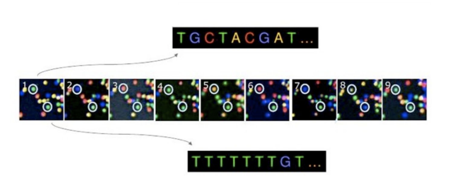
One of the reasons why Illumina sequencers (and similar NGS technologies) have been so successful in the sequencing industry is is that this process is happening across millions of clusters at the same time.

We are hopefully now starting to feel comfortable with the concept for one-colour equals one nucleotide. To throw a curve ball, Illumina sequencers actually have three different ‘colour chemistries’ that they use on different machines.

Colour chemistry

To be able to offer cheaper machines, Illumina came up with alternative systems that require a fewer number of colours to be detected (Fu et al. 2025). These variants are often referred to different ‘colour chemistries’.

A list of Illumina platforms and their colour chemistries (at the time of writing) areas follows below:

• Four-colour chemistry
  • Illumina HiSeq
  • Illumina MiSeq
• Two-colour chemistry
  • Illumina NovaSeq
  • Illumina NextSeq
• One-colour chemistry
  • Illumina iSeq

In the vast majority of cases, our data will be only sequenced on four- and two-colour chemistries, so we will focus on these two.

In the case of the Illumina HiSeq and MiSeq platforms, the system for sequencing is as described previously: each of the four bases of the nucleotides that make up DNA will have a reversible-terminator variant, and each of these variants will have a specific fluorophore that will emit one of four colours. Therefore, the camera on the machine is designed to be able to pick up each of the four different wavelengths through different imaging channels.

In contrast, two-colour chemistry machines will only have imaging channels that detect have two colours - red and green (Figure 1.17). If the machine detects only green being emitted from a cluster on the flowcell, this correspond to T. If the machine detects only red, it records a C. If the machine detects both red and green wavelengths being emitted from a cluster - this corresponds to an A. If no colour is emitted, this is assumed to be a G.

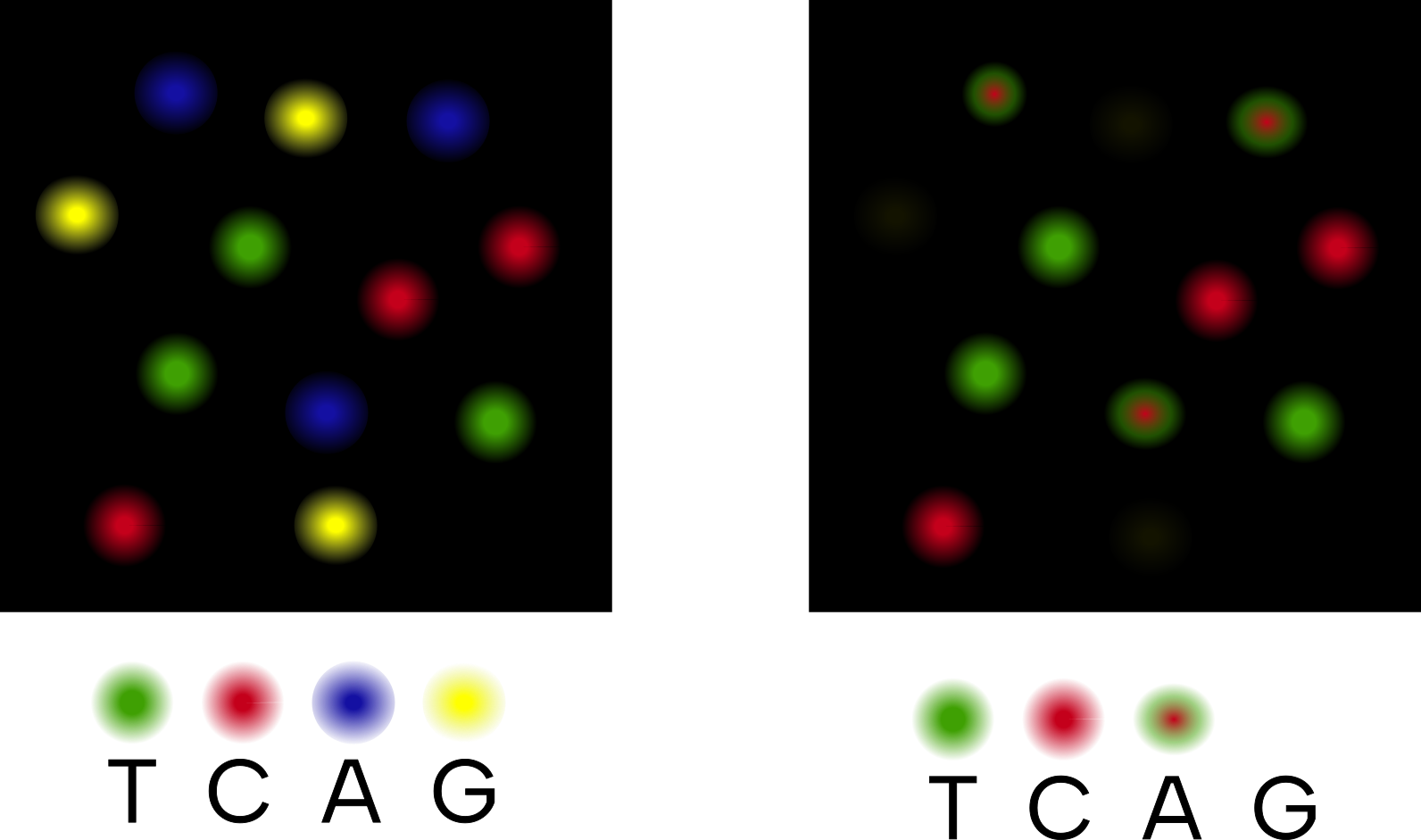
Figure 1.17: Graphical representation of difference between four- (left) and two-colour (right) chemistry of Illumina Platforms. While in four-colour chemistry machines there is one colour for each nucleotide, two colour chemistry models emit single colours for T and C, a mixture of both wavelengths for A, and no colour is assumed to represent a G. Inspired by https://www.ecseq.com/support/ngs/do_you_have_two_colors_or_four_colors_in_Illumina

This characteristic of two colour-chemistry thus means we have to be aware of the type of sequencer our data was generated on, as this will require slightly different computational preprocessing (De-Kayne et al. 2021), as we will see later on in the section on Low sequence diversity.

Base quality and paired-end sequencing

Another consideration with Illumina sequencing kits is not just the number of cycles, but what ‘pairment’ they kit has.

As we all know, biology is not like physics where everything is perfect and ‘logical’ ³. Biology likes to be messy, and things often do not stay consistent.

The same applies to sequencing - as the sequencer goes through each cycle of adding a new nucleotide to each DNA strand in a cluster, ‘mistakes’ will increasingly start to happen (Metzker 2010). Polymerases will not bind properly, or fall off, or skip nucleotides, or even add the wrong base. The accumulated effects of these mistakes across all DNA strands in a cluster is that the emitted light during the imaging part of the cycle becomes less clearly one colour, as mixtures of wavelengths are emitted. This results in our confidence that correct nucleotide has been recorded at a given position of the DNA molecule becomes lower.

Sequencers address this in two ways.

Firstly, when measuring the particular base being recorded, all sequencers will at the same time calculate a ‘base quality’ that is associated with that call (Cacho et al. 2016). This corresponds to the confidence (via a probability) that the recorded base was the correct one. For example, if the wavelength was mostly one colour (let’s say red for C) but the camera picked up a bit of another colour (lets say green for T), it will record C in the output, but the base quality score associated with this base call will be lower. If the sequencer’s camera picks up wavelengths of all four colours from the same cluster at the same time - or even no light is detected at all - then the base quality for that position in that DNA molecule will be recorded as an N and a confidence score of 0.

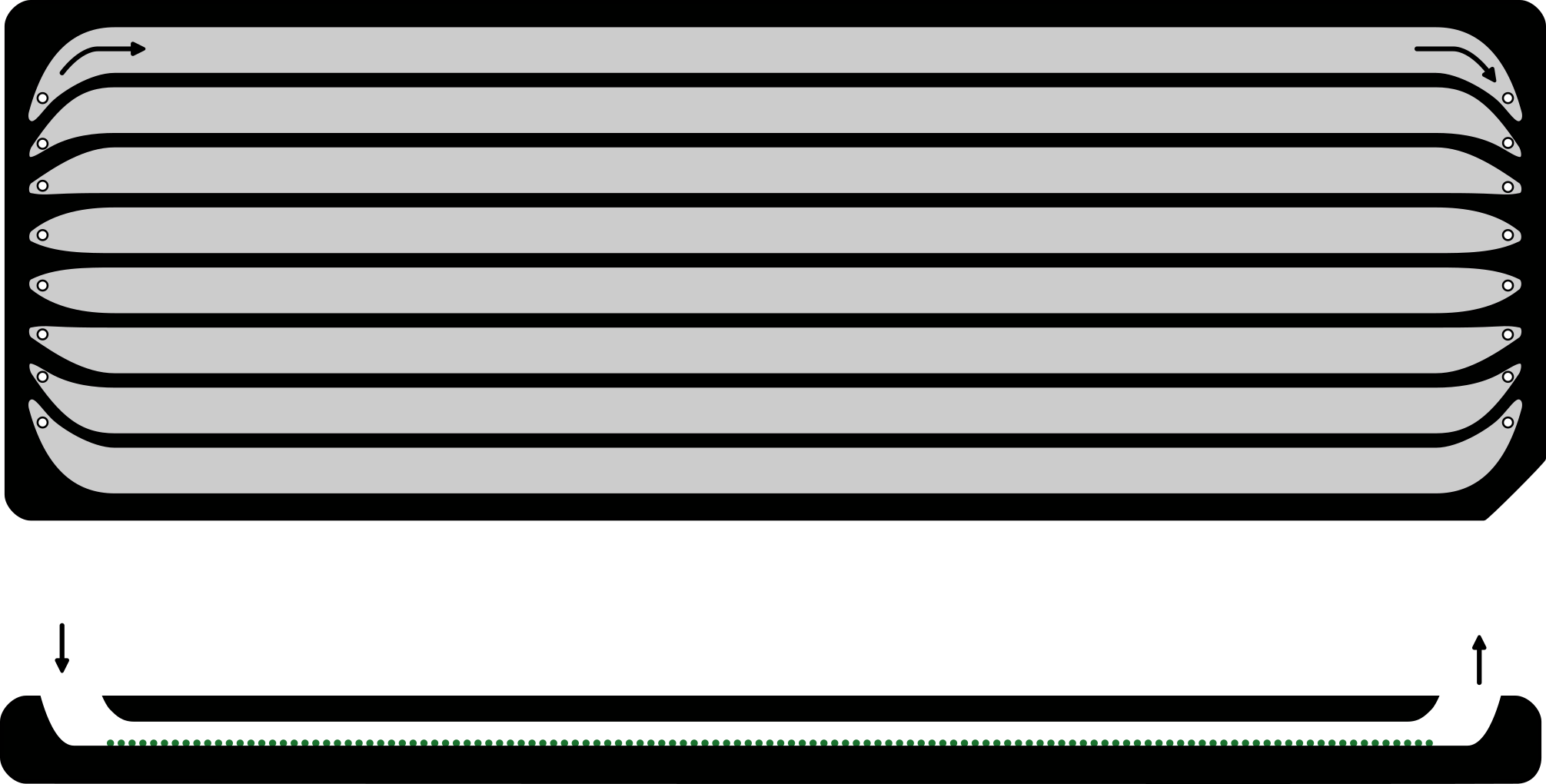
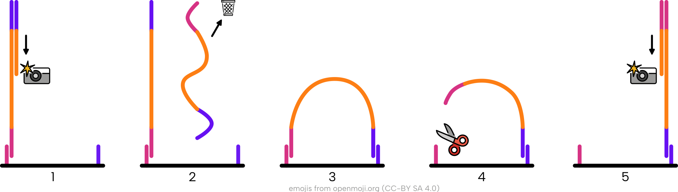
Secondly, specifically for Illumina sequencers, there is the concept of ‘paired-end’ sequencing (Bentley et al. 2008). There is an overall drop in base quality (i.e., confidence we have the right nucleotide) the closer we get to the end of the molecule due to the accumulated mistakes over time. To counteract this, we can freshly sequence the molecule again but in the reverse direction. This way, we can ‘merge’ and take an average of the two base quality scores of two independent ‘observations’ of the nucleotide at a given position. So if the last base when reading the molecule in the forward direction is an N (due to ambiguous wavelength emission), we can correct or ‘recover’ this last base by making it the first base we call in when sequencing in the reverse direction from scratch with fresh reagents.

This works as Illumina sequencers can conveniently re-use the ‘bending over’ approach as performed by the ‘bridge’ amplification method during clustering we saw earlier in this chapter.

In other words, after bending over, the opposite flowcell oligo from the forward reverse flowcell anchor is cut so the ‘end’ of the original molecule is now bound to the flow cell and becomes the ‘start’ of the new cluster (Figure 1.18). This paired-end sequencing technique means we get a pair of files - both with the same sequence from each cluster, but one has the molecule ‘read’ in the forward direction, and the other file with the ‘reverse’ direction.

Another added benefit of paired-end sequencing is that we can recover longer molecules (Magoč and Salzberg 2011). In cases where the DNA molecule is longer than the number of cycles of the chemistry kit, by flipping over the molecule and sequencing from the other end, we can recover the end of the molecule that otherwise falls outside the original number of cycles. Of course, if the molecule is longer than the sum of both set of cycles (e.g. a 120bp molecule, even though the sequencing kit is only two times 50bp), we will still miss the ‘middle’ part of the molecule. However, this is counteracted by the sheer number of independent molecules sequenced, so the ‘missing’ part can be filled in from another sequencing DNA molecule that ‘starts’ in this position.

Figure 1.18: Diagram showing a broad overview of how Illumina paired-end sequencing works for a single DNA molecule. 1. The single-stranded DNA strand is attached to the flow cell, and read in one direction. 2. The molecule is denatured and one strand gets discarded. 3. The molecule is bent over (similar to bridge amplification), and the adapter at the other end is bound to the flow cell. 4. The original anchored end of the molecule is then cut, allowing the original ‘end’ to become the new starting point sequencing. 5. The molecule is sequenced in the reverse direction. Emojis from openmoji.org (CC-BY SA 4.0).

It should be noted, however, that the added benefit of sequencing longer molecules via paired-end sequencing is not always relevant to older ancient DNA or ancient metagenomics. This is because most ‘true’ DNA molecules are often shorter than the sequencing cycles of a typical Illumina kit. That said, fragmented ancient DNA molecules follow a distribution of molecule lengths, and retrieval of longer reads can be useful during in analyses such as de novo assembly for scaffolding purposes (Ayling, Clark, and Leggett 2020).

Base calling and demultiplexing

We now understand how the machine itself ‘reads’ the DNA molecule clusters on the flow cell.

But how do these images get converted to a format that we can read on our computer screens? Furthermore, if we have sequenced multiple samples at the same time with multiplexing (each with their own sample-specific indices), how do we separate the molecules from sample out?

We can do this with two, often integrated, steps.

Base calling is the process of converting the images to digital text-based A, C, T, and Gs (Rougemont et al. 2008). This is not something the vast majority of researchers have to do, as nowadays it happens on the sequencer itself or by the sequencing technicians and thus not necessary for researchers to carry out.

However, once the file with the digital representations of the sequences is taken off the machine, and if not also performed by the sequencing facility, we may have to perform something called ‘demultiplexing’ (Figure 1.19). This involves using computational software that identifies the known index sequence at the beginning of each sequence entry in the base-called file, and then separates all reads containing the same sample-specific index into it’s own independent file.

Figure 1.19: Schematic diagram showing the demultimultiplexing concept. Multiple libraries have been sequenced in a single lane of a sequencer. Each library has their own index sequence combination. Demultiplexing consists of taking the large single-lane FASTQ file, and using information recorded during the library construction to assign each read to it’s associated sample. These reads then are sorted by sample and separated into separate per-sample FASTQ files.

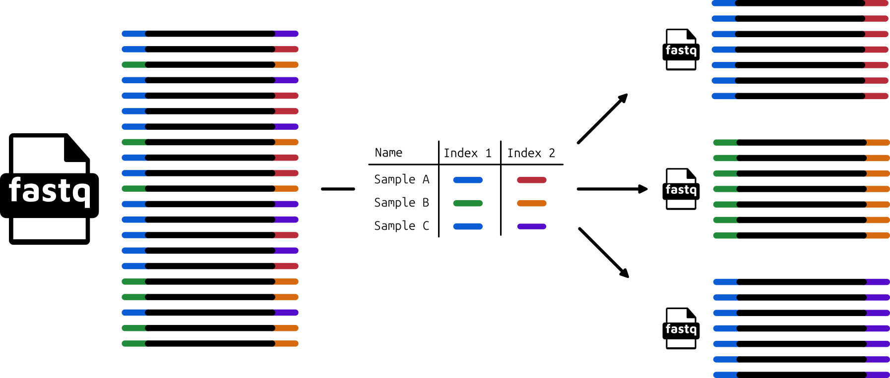
While these processes are not something most researchers will do themselves, it is useful to know the basic concept, as sometimes errors detected in downstream analysis can be traced back to suboptimal demultiplexing. One example is when we have not received the number of reads we expected, which may have be caused by incorrect assignment of indices during demultiplexing.

FASTQ File

The primary output from demultiplexing is called the FASTQ file. This is a text-based (semi-)standard format for storing biological sequences, and their corresponding base quality scores (Cock et al. 2010). A biological sequence that has been converted to a digital text format is referred to as a ‘read’ or ‘sequence read’. The files that store reads are typically compressed to save space, but can still be very large (gigabytes in size, even when compressed).

The structure of a FASTQ file is a repeated series of four lines (Figure 1.20):

1. A metadata or ID line
2. The DNA sequence itself
3. A ‘spacer’ line
4. The base quality score (corresponding to the base in the same position as in line 2)

This can broken down as follows:

The metadata line records a range of information from the sequencer and also potentially the demultiplexing. Typically this line will record the sequencing machine ID, a run number, the ID of the flow cell, coordinate information from which cluster on the flow cell the sequence is from, and then extra information that depends on the sequencing center (e.g., some will record the sample-specific index pairs here, or certain settings of the demultiplexing tool).

Figure 1.20: Annotated example of a single sequencing read as represented in a FASTQ file. A read consists of four lines: a metadata line, a sequence line, a spacer line, and a base quality score line. This set of four lines is repeated for every sequenced molecule in the library. Emojis from openmoji.org (CC-BY SA 4.0)

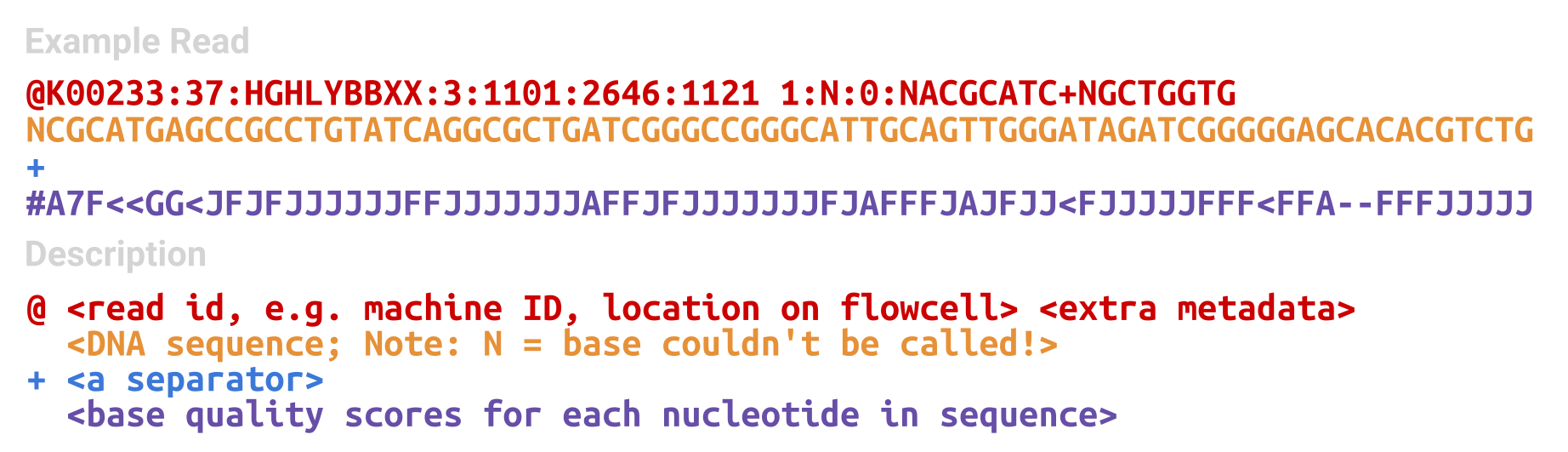
The sequence line will contain A, C, T, G, and N characters in the order of the DNA molecule as recorded by the sequencer. In the figure we can see an example of an N call in the first position ⁴.

The third line is simply a spacer line, which is just a + sign. It serves no purpose in modern day FASTQ files (they just display the + to ensure we retain an even number of lines for analysis purposes), however in the past, the metadata information was duplicated on this line to associate with the base quality scores on line 4.

The fourth line has the base quality scores corresponding to the sequence in line 2. These are encoded using ASCII characters, to allow encoding of scores more than 9 in a single character. What the exact each ASCII character represents slightly depends on which sequencing machine we are using (e.g. Illumina have both a 1.3 and 1.8 variant). However all variants encode a quality score of ‘Q’, also known as a ‘Phred’ score, which corresponds to the probability that the called base is incorrect (Ewing and Green 1998). This essentially means that the lower the probability the base is incorrect, the higher the quality score. Modern Illumina sequencers have a minimum quality score of 0 (i.e., an incorrect call) and a maximum score of 41 (a highly confident call). Wikipedia provides a very good summary of the differences between ASCII representations of the Phred score on different platforms here.

The rest of a FASTQ file is simply just a repeated set of these four lines. Each line corresponds to an independent DNA cluster - and thus DNA molecule - that was sequenced. In the case of Illumina pair-end sequencing, we will normally have two FASTQ files for each sample - and we can match the forward and reverse reading of each strand by the metadata line and a /1 or /2 at the end of the ID⁵.

1.3 Sequencing and considerations for ancient metagenomics

In the second half of this chapter, we will look into some implications of the sequencing process for analysing ancient metagenomic data.

While some of these points are not always specific to ancient metagenomics, and can apply to any DNA analysis - modern or ancient, they can be particularly impactful due to the particular characteristics of ancient DNA.

Low DNA preservation

One side effect of the degradation and lost of DNA molecules in ancient samples is that the total molecular biomass of the sample is very low (Weyrich et al. 2019).

This means that during library preparation, researchers often have to perform many rounds of PCR amplification to get a sufficient library concentration for sequencing.

By over-amplifying libraries, we reduce the number of unique sequences from our sample we can actually retrieve. If we are repeatedly sequencing the same DNA sequence (i.e. the amplified copies) over and over, we use up the fixed number of available clusters on the flow cell (Gloor et al. 2017), and prevent clusters of unique sequences from forming and thus being sequenced.

This is also important analysis-wise, as will be discussed in the chapters on taxonomic profiling and genomic mapping, as we can actually artificially ‘inflate’ the counts of reads that come from a particular taxon (Figure 1.21). For microbiome studies, this can skew the estimate of which species are in our sample or not. Some studies have also suggested dedeuplication can improve the accuracy of metagenomic de novo assembly (Zhang et al. 2023)

Figure 1.21: Schematic representation of the result on over-amplification on reference-based genome mapping. Exact duplicate reads (yellow), that derive from overamplifying a library, can result in portions of the genome having higher depth coverage in certain regions (top distribution) and thus artificially provide a misleading sense of confidence in recovered regions during analysis, even though the overall coverage is low.

While this artefact can be partially corrected during computational analysis through the process of ‘deduplication’, we should be careful and aim to not overamplify our libraries in the first place, as we can potentially waste a lot of money on sequencing uninformative molecules (Daley and Smith 2013).

Index hopping

A more recent artefact that has appeared in more recent Illumina platforms is something that has been termed ‘index hopping’ (T. van der Valk et al. 2019). This can cause problems when we are multiplex-sequencing samples, i.e., sequencing multiple samples at once on the same flow cell.

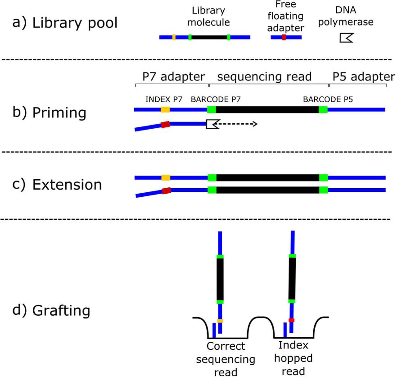
Some more recent Illumina platforms such as the HiSeq X and NovaSeq machines have a new type of flow cell called ‘patterned flow cells’. These aim to better separate out and make more consistent the layout of DNA clusters on the flow cell by having ‘nanowells’ that the clusters form inside. By having a stricter pattern where clusters form, it allows even tighter distribution of clusters on the flow cell without impeding each other and thus increasing the number of clusters that can be sequenced at once (Modi et al. 2021).

However, even though the cause it not fully understood, it appears that the method used to prevent two DNA molecules occupying the same well (‘exclusion amplification’) can accidentally cause ‘switching’ of the index barcode between two different DNA molecules (Figure 1.22). Thus, DNA molecules from one sample can instead receive the index barcode of another sample, and subsequently assigned to the wrong sample during demultiplexing.

While this has been observed a low rates in earlier Illumina platforms, index misassignment appears to occur more often in patterned flow cells, at a rate somewhere between 0%-10% (T. van der Valk et al. 2019).

For (ancient) metagenomics this can be problematic as it can result in false positive identification of taxa in your sample. For example, if you sequence in the same run a capture-library of a pathogen and a shotgun metagenomic library for screening, you may falsely ‘identify’ the presence of the pathogen in the shotgun sample. With index hopping, some of the abundant pathogen reads in the pathogen will be accidentally assigned in demultiplexing to the shotgun metagenomic library giving a false positive identification. In another case, if you have an oral microbiome sample and a gut microbiome sample sequenced on the same run, you may start seeing oral species being detected up in your gut samples. While this could be valid biologically, in other cases this could be false and it becomes hard to disambiguate if the species is truly present in the gut or not.

Figure 1.22: Diagram from T. van der Valk et al. (2018)’s preprint demonstrating how free-floating adapters (with a different index) can be incorrectly incorporated into molecules during exclusion amplification on Illumina platforms using patterned flowcells (reproduced here under a CC-BY-ND 4.0 license without modification).

Therefore, we should always keep this in mind when sending our libraries for sequencing. One workaround to this is to ligate additional (short) ‘inline’ barcodes directly to the DNA molecules during library preparation prior to adding adapters (Rohland et al. 2015). However this adds financial cost, and reduces the length of the template molecule we can sequence (as now we must include the inline barcode in the number of sequencing cycles). Otherwise, good sequencing core facilities will automatically screen for this artefact when using these platforms. Despite this, we should always verify this artefact of the sequencing process has not occurred if we find ‘unexpected’ results in our data.

Sequencing errors

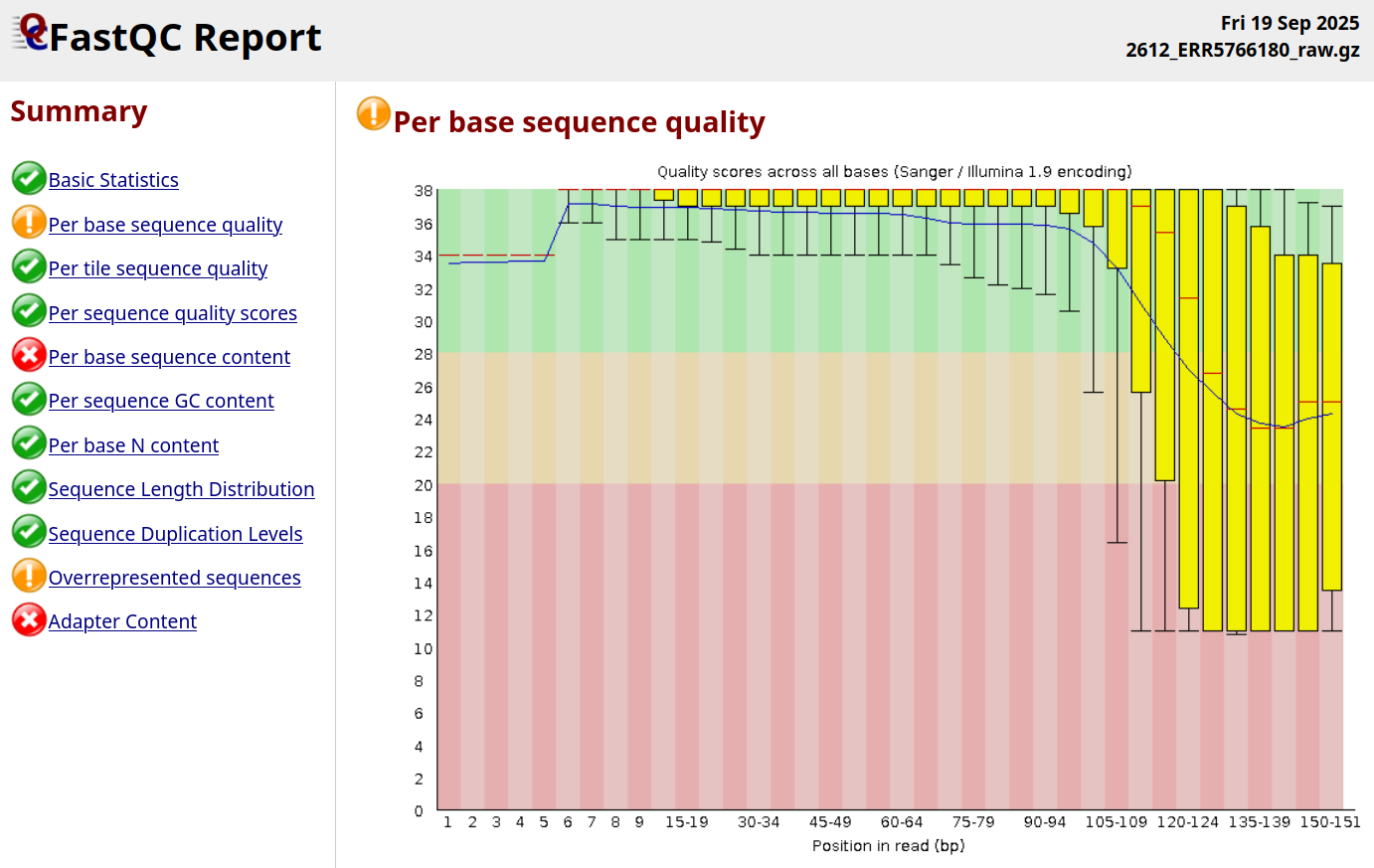
As many parts of this textbook demonstrates, metagenomic sequencing is becoming extremely high-throughput and analysis is becoming increasingly automated and routine. However this does not mean we should skip over quality control of our sequencing data.

While Illumina sequencers nowadays have a very low error rate, they are still not perfect - and things can also go wrong during the sequencing process (Figure 1.23).

All sequencing machines will record ‘their confidence’ in the base calls they make. It is still critical that researchers quality check these before performing downstream analyses.

If our reads have a high number of low base quality socres, the machine may have picked up the wrong nucleotide in the sequence. This could cause a range of problems in various aspects of data analysis: our read may falsely taxonomically classified to the wrong organism with that has a more similar sequence to our errored sequence than the original organism, our read may align to wrong place on a genome during mapping (or not align at all!), prevent sufficient overlap of sequences during assembly causing fragmented assemblies, or even cause false positive variant calls during genotyping for phylogenomic analysis (Dohm et al. 2008).

This is a particular concern for ancient metagenomics due to the very low number of truly endogenous ancient molecules in our libraries. This low number of reads means that we cannot as easily ‘correct’ for errors through simply having many repeated observations of a base call in the same a position (higher depth coverage) from independent DNA molecules.

Many core sequencing facilities will be used to handling modern samples with high quality libraries, and thus the threshold for a rejected sequencing run maybe lower than what we would want for ancient metagenomics. Therefore it’s always important to always (double)check the quality of our sequencing data before proceeding with any analysis.

Figure 1.23: Screenshot of the output of the sequencing quality evaluation tool FASTQC (Andrews 2010) of the ancient DNA palaeofaeces sample 2612 from Maixner et al. (2021). Many of the reads have low quality scores (Y-axis) at the end of molecules (X-axis) from around 110bp. This likely represents error accumulation as the sequencing chemistry becomes ‘tired’. Such low-quality bases should be removed using base quality score trimming to reduce the chance of incorrect read assignment or false-positive variant calls due to the wrong base being called.

Dirty Genomes

Another very common problem we encounter in both ancient and modern metagenomics are ‘dirty genomes’.

To briefly jump ahead into the bioinformatic analysis of an ancient metagenomic project, we will often compare our reads against a reference database of genomes. This is done to classify which species’ genome a particular read comes from, and allows us to infer the taxonomic makeup of the sample.

We pull these reference genomes from a range of user-submitted databases, such as the NCBI’s GenBank or RefSeq databases. However, the genomes that are uploaded to these databases are not always of high quality. Some genomes can contain sequences that should not be there, such as adapters, primers, contaminating sequences from other species, or other artefactual sequences (Longo, O’Neill, and O’Neill 2011; Mukherjee et al. 2015; Merchant, Wood, and Salzberg 2014; Steinegger and Salzberg 2020; Breitwieser et al. 2019; Kryukov and Imanishi 2016). While the NCBI does have quality control checks in place, these have not always been as stringent in the past, and are constantly evolving.

A common example of a notoriously contaminated genome, which many ancient metagenomicists have encountered is the repeated identification of Cyprinus carpio (carp) in their samples (Figure 1.24).

This is not a true hit, but in fact false positive hits due to the presence of adapter sequences in the carp genome ⁶. I.e., remaining adapter sequences in the sequencing library that were not properly removed during read preprocessing, align against the adapter sequences in the carp genome, resulting in false positive identification of carp in all samples.

Figure 1.24: Screenshot of the exasperation after the discovery of a publicly available Cyprinus carpio (carp) genome that was full of sequencing adapters. Any remaining sequencing adapters in our FASTQ files would thus align against the sequences in this genome and we would magically have carp in all of our metagenomic samples. Screenshot of post on the Opinionomics blog by Mick Watson

The implication for ancient metagenomicists is that if we do not properly remove artefacts from our reads, we can end up with a lot of false positive hits in our data. This can be particularly impactful, for example, if we are trying to identify the presence of dietary species in a human microbiome sample. But this also extends to microbes, where insufficient removal of contaminating DNA (e.g. modern human sequences incorporated during sampling) can align against stretches of human sequences incorporated into chimeric reference microbial genomes Gihawi et al. (2023).

Therefore, while it is always good to perform quality checks on the genomes going into our reference database, we should also thoroughly quality control our sequenced reads prior downstream analysis. We should make sure to trim reads of adapters, remove host contamination and other artefacts, and check these steps worked properly!

Low Sequence Diversity Reads

The presence of low sequence diversity reads in a FASTQ file can cause degraded computational performance, and skew higher-level taxonomic assignments.

Low sequence diversity reads are those that have very little nucleotide variation, such as mononucleotide (GGGGGG) or dinucleotide (ATATAT) repeats. While some of these are not necessarily errors (long stretches of repeats do occur naturally in particularly eukaryotic genomes), they can also be caused by the type of sequencer used.

As described earlier in this chapter, Illumina NovaSeq and NextSeq platforms use two-colour chemistry. In this system, if no light is detected by the camera, the sequencer assumes the base is a G. Therefore if the molecule is very short, once the molecule finishes and there are still remaining sequencing cycles to go, there will be repeated cycles of no light being emitted ⁷. This results in poly-G ‘tails’ in reads.

Ancient DNA libraries are particularly susceptible to poly-G tails, as the degraded nature of the molecules means that a large number of are very short and thus the length of molecule finishes before all the cycles have finished.

The impact of these low sequence diversity reads is two-fold. Firstly, they slow down processing of reads during the computationally expensive step of alignment to eukaryotic genomes, as low sequence diversity reads can often match many different locations on ta genome, and thus result in an unspecific or ambiguous alignment. These often do not provide useful information, and are anyway discarded during downstream analysis - but only after the computational resources have been used to align them in the first place. Secondly, we can also end up losing otherwise valid reads, purely due to half of the read having an artefactual stretch of nucleotides at the tail end (e.g. AGTCTCGATGGGGGGGGGG, where the first half is a valid sequence and the tail is just because the sequence is short) and thus cannot be aligned to any part of a reference genome. For taxonomic profiling, reads that match multiple genomes will be pushed by Lowest Common Ancestor algorithms ‘up’ the taxonomic tree. When comparing taxonomic profiles between samples at higher ranks, this can inflate counts at higher nodes (e.g., kingdom or phylum level) that do not accurately reflect the true diversity of the sample, as ultimately such reads are sequencing artefacts.

Therefore, if we have sequencing data (particularly from Illumina two-colour chemistry platforms), it is a good idea to check for signatures of increased low sequence diversity reads and remove these from our data through poly-G trimming. Read processing tools such as fastp (Chen et al. 2018) can help with this, as they have functionality that can automatically detect and remove poly-G tails from reads.

1.4 Summary

In this chapter we have covered how the structure of DNA molecules and process of replication is critical to understanding how genetic sequencing works.

We looked at how library preparation is required to add adapters that can include sample specific barcodes to immobilise DNA molecules to the flow cell. We also went through the differences between four- and two-colour Illumina sequencing chemistry, which differ on how each nucleotide added emits a light captured by a camera.

We discussed how sequencing methods are not perfect, and how the confidence in base calls are stored in FASTQ files, and how such low confidence calls can be corrected through paired-end sequencing.

Finally we discussed some important considerations ancient DNA and ancient metagenomics, including duplicated sequences, index hopping, sequencing errors, causes behind contaminated reference genomes, and poly-G tails in low sequence diversity reads.

1.5 Questions to think about

• Why is Illumina sequencing technologies useful for aDNA?
• What problems can the four-colour chemistry technology of NextSeq and NovaSeqs cause in downstream analysis?
• Why is ‘Index-Hopping’ a problem?
• What is good software to evaluate the quality of your sequencing runs?

1.6 References

Andreeva, T V, A B Malyarchuk, A D Soshkina, N A Dudko, M Yu Plotnikova, and E I Rogaev. 2022. “Methodologies for Ancient DNA Extraction from Bones for Genomic Analysis: Approaches and Guidelines.” Russian Journal of Genetics 58 (9): 1017–35. https://doi.org/10.1134/s1022795422090034.

Andrews, Simon. 2010. “FastQC: A Quality Control Tool for High Throughput Sequence Data.” http://www.bioinformatics.babraham.ac.uk/projects/fastqc/.

Ayling, Martin, Matthew D Clark, and Richard M Leggett. 2020. “New Approaches for Metagenome Assembly with Short Reads.” Briefings in Bioinformatics 21 (2): 584–94. https://doi.org/10.1093/bib/bbz020.

Bentley, David R, Shankar Balasubramanian, Harold P Swerdlow, Geoffrey P Smith, John Milton, Clive G Brown, Kevin P Hall, et al. 2008. “Accurate Whole Human Genome Sequencing Using Reversible Terminator Chemistry.” Nature 456 (7218): 53–59. https://doi.org/10.1038/nature07517.

Breitwieser, Florian P, Mihaela Pertea, Aleksey Zimin, and Steven L Salzberg. 2019. “Human Contamination in Bacterial Genomes Has Created Thousands of Spurious Proteins.” Genome Research 29 (May): 954–60. https://doi.org/10.1101/gr.245373.118.

Bronner, Iraad F, Michael A Quail, Daniel J Turner, and Harold Swerdlow. 2013. “Improved Protocols for Illumina Sequencing.” Et Al [Current Protocols in Human Genetics] 79 (1): 18.2.1–42. https://doi.org/10.1002/0471142905.hg1802s79.

Cacho, Ashley, Ekaterina Smirnova, Snehalata Huzurbazar, and Xinping Cui. 2016. “A Comparison of Base-Calling Algorithms for Illumina Sequencing Technology.” Briefings in Bioinformatics 17 (5): 786–95. https://doi.org/10.1093/bib/bbv088.

Chen, Shifu, Yanqing Zhou, Yaru Chen, and Jia Gu. 2018. “Fastp: An Ultra-Fast All-in-One FASTQ Preprocessor.” Bioinformatics 34 (17): i884–90. https://doi.org/10.1093/bioinformatics/bty560.

Church, G M, and S Kieffer-Higgins. 1988. “Multiplex DNA Sequencing.” Science (New York, N.Y.) 240 (4849): 185–88. https://doi.org/10.1126/science.3353714.

Cock, Peter J A, Christopher J Fields, Naohisa Goto, Michael L Heuer, and Peter M Rice. 2010. “The Sanger FASTQ File Format for Sequences with Quality Scores, and the Solexa/Illumina FASTQ Variants.” Nucleic Acids Research 38 (6): 1767–71. https://doi.org/10.1093/nar/gkp1137.

Dabney, Jesse, Matthias Meyer, and Svante Pääbo. 2013. “Ancient DNA Damage.” Cold Spring Harbor Perspectives in Biology 5 (7). https://doi.org/10.1101/cshperspect.a012567.

Daley, Timothy, and Andrew D Smith. 2013. “Predicting the Molecular Complexity of Sequencing Libraries.” Nature Methods 10 (4): 325–27. https://doi.org/10.1038/nmeth.2375.

Danaeifar, Mohsen. 2022. “New Horizons in Developing Cell Lysis Methods: A Review.” Biotechnology and Bioengineering 119 (11): 3007–21. https://doi.org/10.1002/bit.28198.

De-Kayne, Rishi, David Frei, Ryan Greenway, Sofia L Mendes, Cas Retel, and Philine G D Feulner. 2021. “Sequencing Platform Shifts Provide Opportunities but Pose Challenges for Combining Genomic Data Sets.” Molecular Ecology Resources 21 (3): 653–60. https://doi.org/10.1111/1755-0998.13309.

Dohm, Juliane C, Claudio Lottaz, Tatiana Borodina, and Heinz Himmelbauer. 2008. “Substantial Biases in Ultra-Short Read Data Sets from High-Throughput DNA Sequencing.” Nucleic Acids Research 36 (16): e105. https://doi.org/10.1093/nar/gkn425.

Ewing, B, and P Green. 1998. “Base-Calling of Automated Sequencer Traces Using Phred. II. Error Probabilities.” Genome Research 8 (3): 186–94. https://doi.org/10.1101/gr.8.3.186.

Fu, Beverly J, Vinayak V Viswanadham, Dominika Maziec, Hu Jin, and Peter J Park. 2025. “A Recurrent Sequencing Artifact on Illumina Sequencers with Two-Color Fluorescent Dye Chemistry and Its Impact on Somatic Variant Detection.” bioRxiv.org: The Preprint Server for Biology, September, 2025.09.27.678978. https://doi.org/10.1101/2025.09.27.678978.

Gihawi, Abraham, Yuchen Ge, Jennifer Lu, Daniela Puiu, Amanda Xu, Colin S Cooper, Daniel S Brewer, Mihaela Pertea, and Steven L Salzberg. 2023. “Major Data Analysis Errors Invalidate Cancer Microbiome Findings.” mBio 14 (5): e0160723. https://doi.org/10.1128/mbio.01607-23.

Gloor, Gregory B, Jean M Macklaim, Vera Pawlowsky-Glahn, and Juan J Egozcue. 2017. “Microbiome Datasets Are Compositional: And This Is Not Optional.” Frontiers in Microbiology 8 (November): 2224. https://doi.org/10.3389/fmicb.2017.02224.

Heather, James M, and Benjamin Chain. 2015. “The Sequence of Sequencers: The History of Sequencing DNA.” Genomics, November. https://doi.org/10.1016/j.ygeno.2015.11.003.

Holt, Robert A, and Steven J M Jones. 2008. “The New Paradigm of Flow Cell Sequencing.” Genome Research 18 (6): 839–46. https://doi.org/10.1101/gr.073262.107.

Ju, Jingyue, Dae Hyun Kim, Lanrong Bi, Qinglin Meng, Xiaopeng Bai, Zengmin Li, Xiaoxu Li, et al. 2006. “Four-Color DNA Sequencing by Synthesis Using Cleavable Fluorescent Nucleotide Reversible Terminators.” Proceedings of the National Academy of Sciences of the United States of America 103 (52): 19635–40. https://doi.org/10.1073/pnas.0609513103.

Kircher, Martin, Susanna Sawyer, and Matthias Meyer. 2012. “Double Indexing Overcomes Inaccuracies in Multiplex Sequencing on the Illumina Platform.” Nucleic Acids Research 40 (1): e3. https://doi.org/10.1093/nar/gkr771.

Koboldt, Daniel C, Karyn Meltz Steinberg, David E Larson, Richard K Wilson, and Elaine R Mardis. 2013. “The Next-Generation Sequencing Revolution and Its Impact on Genomics.” Cell 155 (1): 27–38. https://doi.org/10.1016/j.cell.2013.09.006.

Kryukov, Kirill, and Tadashi Imanishi. 2016. “Human Contamination in Public Genome Assemblies.” PloS One 11 (9): e0162424. https://doi.org/10.1371/journal.pone.0162424.

Longo, Mark S, Michael J O’Neill, and Rachel J O’Neill. 2011. “Abundant Human DNA Contamination Identified in Non-Primate Genome Databases.” PloS One 6 (2): e16410. https://doi.org/10.1371/journal.pone.0016410.

Magoč, Tanja, and Steven L Salzberg. 2011. “FLASH: Fast Length Adjustment of Short Reads to Improve Genome Assemblies.” Bioinformatics (Oxford, England) 27 (21): 2957–63. https://doi.org/10.1093/bioinformatics/btr507.

Maixner, Frank, Mohamed S Sarhan, Kun D Huang, Adrian Tett, Alexander Schoenafinger, Stefania Zingale, Aitor Blanco-Míguez, et al. 2021. “Hallstatt Miners Consumed Blue Cheese and Beer During the Iron Age and Retained a Non-Westernized Gut Microbiome Until the Baroque Period.” Current Biology: CB, October. https://doi.org/10.1016/j.cub.2021.09.031.

Merchant, Samier, Derrick E Wood, and Steven L Salzberg. 2014. “Unexpected Cross-Species Contamination in Genome Sequencing Projects.” PeerJ 2 (November): e675. https://doi.org/10.7717/peerj.675.

Metzker, Michael L. 2010. “Sequencing Technologies - the Next Generation.” Nature Reviews. Genetics 11 (1): 31–46. https://doi.org/10.1038/nrg2626.

Modi, Alessandra, Stefania Vai, David Caramelli, and Martina Lari. 2021. “The Illumina Sequencing Protocol and the NovaSeq 6000 System.” Bacterial Pangenomics, 15–42. https://doi.org/10.1007/978-1-0716-1099-2\_2.

Mukherjee, Supratim, Marcel Huntemann, Natalia Ivanova, Nikos C Kyrpides, and Amrita Pati. 2015. “Large-Scale Contamination of Microbial Isolate Genomes by Illumina PhiX Control.” Standards in Genomic Sciences 10 (March): 18. https://doi.org/10.1186/1944-3277-10-18.

Rohland, Nadin, Eadaoin Harney, Swapan Mallick, Susanne Nordenfelt, and David Reich. 2015. “Partial Uracil-DNA-Glycosylase Treatment for Screening of Ancient DNA.” Philosophical Transactions of the Royal Society of London. Series B, Biological Sciences 370 (1660): 20130624. https://doi.org/10.1098/rstb.2013.0624.

Rougemont, Jacques, Arnaud Amzallag, Christian Iseli, Laurent Farinelli, Ioannis Xenarios, and Felix Naef. 2008. “Probabilistic Base Calling of Solexa Sequencing Data.” BMC Bioinformatics 9 (1): 431. https://doi.org/10.1186/1471-2105-9-431.

Sanger, F, S Nicklen, and A R Coulson. 1977. “DNA Sequencing with Chain-Terminating Inhibitors.” Proceedings of the National Academy of Sciences of the United States of America 74 (12): 5463–67. https://doi.org/10.1073/pnas.74.12.5463.

Schloss, Jeffery A, Richard A Gibbs, Vinod B Makhijani, and Andre Marziali. 2020. “Cultivating DNA Sequencing Technology After the Human Genome Project.” Annual Review of Genomics and Human Genetics 21 (1): 117–38. https://doi.org/10.1146/annurev-genom-111919-082433.

Shendure, Jay A, Gregory J Porreca, George M Church, Andrew F Gardner, Cynthia L Hendrickson, Jan Kieleczawa, and Barton E Slatko. 2011. “Overview of DNA Sequencing Strategies.” Et Al [Current Protocols in Molecular Biology] Chapter 7 (1): Unit7.1. https://doi.org/10.1002/0471142727.mb0701s96.

Shendure, Jay, and Hanlee Ji. 2008. “Next-Generation DNA Sequencing.” Nature Biotechnology 26 (10): 1135–45. https://doi.org/10.1038/nbt1486.

Steinegger, Martin, and Steven L Salzberg. 2020. “Terminating Contamination: Large-Scale Search Identifies More Than 2,000,000 Contaminated Entries in GenBank.” Genome Biology 21 (1): 115. https://doi.org/10.1186/s13059-020-02023-1.

Valencia, C Alexander, M Ali Pervaiz, Ammar Husami, Yaping Qian, and Kejian Zhang. 2013. “Sanger Sequencing Principles, History, and Landmarks.” In SpringerBriefs in Genetics, 3–11. New York, NY: Springer New York. https://doi.org/10.1007/978-1-4614-9032-6\_1.

Valk, Tom van der, Francesco Vezzi, Mattias Ormestad, Love Dalén, and Katerina Guschanski. 2018. “Index Hopping on the Illumina HiseqX Platform and Its Consequences for Ancient DNA Studies.” bioRxiv. https://doi.org/10.1101/179028.

Valk, Tom van der, Francesco Vezzi, Mattias Ormestad, Love Dalén, and Katerina Guschanski. 2019. “Index Hopping on the Illumina HiseqX Platform and Its Consequences for Ancient DNA Studies.” Molecular Ecology Resources, March. https://doi.org/10.1111/1755-0998.13009.

Weyrich, Laura S, Andrew G Farrer, Raphael Eisenhofer, Luis A Arriola, Jennifer Young, Caitlin A Selway, Matilda Handsley-Davis, Christina J Adler, James Breen, and Alan Cooper. 2019. “Laboratory Contamination over Time During Low-Biomass Sample Analysis.” Molecular Ecology Resources 19 (4): 982–96. https://doi.org/10.1111/1755-0998.13011.

Zhang, Zhiguo, Lu Zhang, Guoqing Zhang, Ze Zhao, Hui Wang, and Feng Ju. 2023. “Deduplication Improves Cost-Efficiency and Yields of DE Novo Assembly and Binning of Shotgun Metagenomes in Microbiome Research.” Microbiology Spectrum, February, e0428222. https://doi.org/10.1128/spectrum.04282-22.

---

1. Newer techniques such as Nanopore sequencers use different methods.

2. With the more recent emergence of Nanopore sequencing, really NGS should be equated to ‘second generation sequencing’, a term you will see in some contexts.

3. Take this statement very much tongue in cheek.

4. It is actually quite common to see in the first or second position of reads, as the sequencer’s camera is still calibrating itself.

5. We can occasionally encounter a format called ‘interleaved’ FASTQ files, where the forward and reverse reads are placed right after one another in the same file, but this is not common practice any more.

6. See https://web.archive.org/web/20170823143538/http://www.opiniomics.org/we-need-to-stop-making-this-simple-fcking-mistake/ and https://web.archive.org/web/20241012070028/https://grahametherington.blogspot.com/2014/09/why-you-should-qc-your-reads-and-your.html

7. See: https://support.illumina.com/content/dam/illumina-support/help/Illumina_DRAGEN_Bio_IT_Platform_v3_7_1000000141465/Content/SW/Informatics/Dragen/PolyG_Trimming_fDG.htm