8 Introduction to Python and Pandas
This session is typically ran held in parallel to the Introduction to R and Tidyverse. Participants of the summer schools chose which to attend based on their prior experience. We recommend the introduction to R session if you have no experience with neither R nor Python.
For this chapter’s exercises, if not already performed, you will need to download the chapter’s dataset, decompress the archive, and create and activate the conda environment.
Do this, use wget or right click and save to download this Zenodo archive: 10.5281/zenodo.8413046, and unpack
tar xvf python-pandas.tar.gz
cd python-pandas/
You can then create the subsequently activate environment with
conda env create -f python-pandas.yml
conda activate python-pandas
8.1 Introduction
Over the last few years, Python has gained popularity thanks to the numerous libraries (packages with pre-written functions) in the field of machine learning, statistical data analysis, and bioinformatics. While a few years ago, it was often necessary to go to R for performing routine data manipulation and analysis tasks, nowadays Python has a vast ecosystem of libraries. Libraries exist for many different file formats that you might encounter in metagenomics, such as fasta, fastq, sam, bam, etc.
This tutorial/walkthrough will provide a short introduction to the most popular libraries for data analysis pandas. This library has functions for reading and manipulating tabular data similar to the data.frame() in R together with some basic data plotting codes.
The aim of this walkthrough is to first: get familiar with the Python code syntax and use Jupiter Notebook for executing codes and secondly get a kickstart to utilising the endless possibilities of data analysis in Python that can be applied to your data.
8.2 Working in a jupyter environment
This tutorial run-through is using a Jupyter Notebook for writing & executing Python code and for annotating.
Jupyter notebooks are convenient and have two types of cells: Markdown and Code. The markup cell syntax is very similar to R markdown. The markdown cells are used for annotating, which is important for sharing code with collaborators, reproducibility, and documentation.
To load, please run the following command from within the chapter’s directory.
jupyter notebookThe in the folder tree, navigate to the python-pandas_lecture directory, and then open the student-notebook.ipynb.
You can then follow that notebook, which should mirror the contents of this chapter! Otherwise try making a new notebook within Jupyter File > New > Notebook!
If you get stuck on solutions to the tasks in the Jupyter notebook, the answers should be in the corresponding ‘Solutions’ chapter on this page.
A few examples are shown below. For a full list of possible syntax click here for a Jupyter Notebook cheat-sheet.
list of markdown cell examples:
In many cases, there are multiple possible syntaxes which give the same result. We present only one way in this run-through.
Text
**bold**: bold*italics*: italics
Code
- `inline code` :
inline code
LaTeX maths
$ x = \frac{\pi}{42} $: \[ x = \frac{\pi}{42} \]
url links
[link](https://www.python.org/)link
Images

The code cells can interpret many different coding languages including Python and Bash. The syntax of the code cells is the same as the syntax of the coding languages, in our case python.
Below are some examples of Python code cells with some useful basic python functions:
print() is a python function for printing lines in the terminal print() == echo in bash
print("Hello World from Python!")out - Hello World from Python!
But it can also, for example, run bash commands by adding a ! at the start of the line.
! echo "Hello World from bash!"out - Hello World from bash!
Stings or numbers can be stored as a variable by using the = sign
i = 0Ones a variable is set in one code cell they are stored and can be accessed in other downstream code cells.
print(i)You can also print multiple things together in one print statement such as a number and a string:
print("The number is", i, "Wow!")out - The number is 0 Wow!
8.3 Pandas
8.3.1 Getting started
Pandas is a Python library used for data manipulation and analysis.
We can import the library like this:
import pandas as pdWe set “pandas” to the alias “pd” because we are lazy and don’t want to write the full word too many times.
Now, we can print the current version:
pd.__version__out - '2.0.1'
8.3.2 Pandas data structures
The primary data structures in Pandas are Series and DataFrame.
A DataFrame is a table with columns and rows.
Each column has a column name and each row has an index.

A single row or column (1 dimensional data) is a Series.

For a more in detail pandas getting started tutorial click here
8.4 Reading data with Pandas
Pandas can read in csv (comma separated values) files, which are tables in text format.
It’s called csv because each value is separated from the others via a comma, like this:
A,B
5,6
8,4| A | B | |
|---|---|---|
| 1 | 2 | 3 |
| 2 | 3 | 4 |
Another common tabular separator are tsv, where each value is separated by a tab \t
A\tB
5\t6
8\t4
Our dataset
"all_data.tsv"is tab separated, which Pandas can handle using thesepargument.
pd.read_csv() is the pandas function to read in tabular tables. The sep= can be specified argument, sep=, is the default.
df = pd.read_csv("../all_data.tsv", sep="\t")
df| ID | Year_Birth | Education | Marital_Status | Income | Kidhome | Teenhome | MntWines | MntFruits | MntMeatProducts | MntFishProducts | MntSweetProducts | MntGoldProds | NumWebPurchases | NumCatalogPurchases | NumStorePurchases | NumWebVisitsMonth | Complain | Z_CostContact | Z_Revenue | |
|---|---|---|---|---|---|---|---|---|---|---|---|---|---|---|---|---|---|---|---|---|
| 0 | 5524 | 1957 | Graduation | Single | 58138.0 | 0 | 0 | 635 | 88 | 546 | 172 | 88 | 88 | 8 | 10 | 4 | 7 | 0 | 3 | 11 |
| 1 | 2174 | 1954 | Graduation | Single | 46344.0 | 1 | 1 | 11 | 1 | 6 | 2 | 1 | 6 | 1 | 1 | 2 | 5 | 0 | 3 | 11 |
| 2 | 4141 | 1965 | Graduation | Together | 71613.0 | 0 | 0 | 426 | 49 | 127 | 111 | 21 | 42 | 8 | 2 | 10 | 4 | 0 | 3 | 11 |
| 3 | 6182 | 1984 | Graduation | Together | 26646.0 | 1 | 0 | 11 | 4 | 20 | 10 | 3 | 5 | 2 | 0 | 4 | 6 | 0 | 3 | 11 |
| 4 | 7446 | 1967 | Master | Together | 62513.0 | 0 | 1 | 520 | 42 | 98 | 0 | 42 | 14 | 6 | 4 | 10 | 6 | 0 | 3 | 11 |
| … | … | … | … | … | … | … | … | … | … | … | … | … | … | … | … | … | … | … | … | … |
| 1749 | 9432 | 1977 | Graduation | Together | 666666.0 | 1 | 0 | 9 | 14 | 18 | 8 | 1 | 12 | 3 | 1 | 3 | 6 | 0 | 3 | 11 |
| 1750 | 8372 | 1974 | Graduation | Married | 34421.0 | 1 | 0 | 3 | 3 | 7 | 6 | 2 | 9 | 1 | 0 | 2 | 7 | 0 | 3 | 11 |
| 1751 | 10870 | 1967 | Graduation | Married | 61223.0 | 0 | 1 | 709 | 43 | 182 | 42 | 118 | 247 | 9 | 3 | 4 | 5 | 0 | 3 | 11 |
| 1752 | 7270 | 1981 | Graduation | Divorced | 56981.0 | 0 | 0 | 908 | 48 | 217 | 32 | 12 | 24 | 2 | 3 | 13 | 6 | 0 | 3 | 11 |
| 1753 | 8235 | 1956 | Master | Together | 69245.0 | 0 | 1 | 428 | 30 | 214 | 80 | 30 | 61 | 6 | 5 | 10 | 3 | 0 | 3 | 11 |
1754 rows × 20 columns
When you are unsure what arguments a function can take, it is possible to get a help documentation using help(pd.read_csv)
8.5 Data exploration
The data is from a customer personality analysis of a company trying to better understand how to modify their product catalogue. Here is the link to the original source for more information.
8.5.1 Columns
The command below prints all the column names.
df.columnsIndex(['ID', 'Year_Birth', 'Education', 'Marital_Status', 'Income', 'Kidhome',
'Teenhome', 'MntWines', 'MntFruits', 'MntMeatProducts',
'MntFishProducts', 'MntSweetProducts', 'MntGoldProds',
'NumWebPurchases', 'NumCatalogPurchases', 'NumStorePurchases',
'NumWebVisitsMonth', 'Complain', 'Z_CostContact', 'Z_Revenue'],
dtype='object')We can also list their respective data types.
int64are integersfloat64are floating point numbers, also calleddoublein other languagesobjectare Python objects, which are strings in this case
df.dtypesID int64
Year_Birth int64
Education object
Marital_Status object
Income float64
Kidhome int64
Teenhome int64
MntWines int64
MntFruits int64
MntMeatProducts int64
MntFishProducts int64
MntSweetProducts int64
MntGoldProds int64
NumWebPurchases int64
NumCatalogPurchases int64
NumStorePurchases int64
NumWebVisitsMonth int64
Complain int64
Z_CostContact int64
Z_Revenue int64
dtype: object8.5.2 Inspecting the DataFrame
What is the size of our DataFrame
df.shape(1754, 20)It has 1754 rows and 20 columns.
Let’s look at the first 5 rows:
df.head()| ID | Year_Birth | Education | Marital_Status | Income | Kidhome | Teenhome | MntWines | MntFruits | MntMeatProducts | MntFishProducts | MntSweetProducts | MntGoldProds | NumWebPurchases | NumCatalogPurchases | NumStorePurchases | NumWebVisitsMonth | Complain | Z_CostContact | Z_Revenue | |
|---|---|---|---|---|---|---|---|---|---|---|---|---|---|---|---|---|---|---|---|---|
| 0 | 5524 | 1957 | Graduation | Single | 58138.0 | 0 | 0 | 635 | 88 | 546 | 172 | 88 | 88 | 8 | 10 | 4 | 7 | 0 | 3 | 11 |
| 1 | 2174 | 1954 | Graduation | Single | 46344.0 | 1 | 1 | 11 | 1 | 6 | 2 | 1 | 6 | 1 | 1 | 2 | 5 | 0 | 3 | 11 |
| 2 | 4141 | 1965 | Graduation | Together | 71613.0 | 0 | 0 | 426 | 49 | 127 | 111 | 21 | 42 | 8 | 2 | 10 | 4 | 0 | 3 | 11 |
| 3 | 6182 | 1984 | Graduation | Together | 26646.0 | 1 | 0 | 11 | 4 | 20 | 10 | 3 | 5 | 2 | 0 | 4 | 6 | 0 | 3 | 11 |
| 4 | 7446 | 1967 | Master | Together | 62513.0 | 0 | 1 | 520 | 42 | 98 | 0 | 42 | 14 | 6 | 4 | 10 | 6 | 0 | 3 | 11 |
What we can see it that, unlike R, Python and in extension Pandas is 0-indexed instead of 1-indexed.
Question: Can you show how to do the same using bash?
! head all_data.tsv| ID | Year_Birth | Education | Marital_Status | Income | Kidhome | Teenhome | MntWines | MntFruits | MntMeatProducts | MntFishProducts | MntSweetProducts | MntGoldProds | NumWebPurchases | NumCatalogPurchases | NumStorePurchases | NumWebVisitsMonth | Complain | Z_CostContact | Z_Revenue | |
|---|---|---|---|---|---|---|---|---|---|---|---|---|---|---|---|---|---|---|---|---|
| 0 | 5524 | 1957 | Graduation | Single | 58138.0 | 0 | 0 | 635 | 88 | 546 | 172 | 88 | 88 | 8 | 10 | 4 | 7 | 0 | 3 | 11 |
| 1 | 2174 | 1954 | Graduation | Single | 46344.0 | 1 | 1 | 11 | 1 | 6 | 2 | 1 | 6 | 1 | 1 | 2 | 5 | 0 | 3 | 11 |
| 2 | 4141 | 1965 | Graduation | Together | 71613.0 | 0 | 0 | 426 | 49 | 127 | 111 | 21 | 42 | 8 | 2 | 10 | 4 | 0 | 3 | 11 |
| 3 | 6182 | 1984 | Graduation | Together | 26646.0 | 1 | 0 | 11 | 4 | 20 | 10 | 3 | 5 | 2 | 0 | 4 | 6 | 0 | 3 | 11 |
| 4 | 7446 | 1967 | Master | Together | 62513.0 | 0 | 1 | 520 | 42 | 98 | 0 | 42 | 14 | 6 | 4 | 10 | 6 | 0 | 3 | 11 |
| 5 | 965 | 1971 | Graduation | Divorced | 55635.0 | 0 | 1 | 235 | 65 | 164 | 50 | 49 | 27 | 7 | 3 | 7 | 6 | 0 | 3 | 11 |
| 6 | 1994 | 1983 | Graduation | Married | NaN | 1 | 0 | 5 | 5 | 6 | 0 | 2 | 1 | 1 | 0 | 2 | 7 | 0 | 3 | 11 |
| 7 | 387 | 1976 | Basic | Married | 7500.0 | 0 | 0 | 6 | 16 | 11 | 11 | 1 | 16 | 2 | 0 | 3 | 8 | 0 | 3 | 11 |
| 8 | 2125 | 1959 | Graduation | Divorced | 63033.0 | 0 | 0 | 194 | 61 | 480 | 225 | 112 | 30 | 3 | 4 | 8 | 2 | 0 | 3 | 11 |
| 9 | 8180 | 1952 | Master | Divorced | 59354.0 | 1 | 1 | 233 | 2 | 53 | 3 | 5 | 14 | 6 | 1 | 5 | 6 | 0 | 3 | 11 |
8.5.3 Accessing rows and columns
We can access parts of the data in DataFrames in different ways.
The first method is sub-setting the rows using the index.
This will take only the second row and all columns, producing a Series:
df.loc[1, :]ID 2174
Year_Birth 1954
Education Graduation
Marital_Status Single
Income 46344.0
Kidhome 1
Teenhome 1
MntWines 11
MntFruits 1
MntMeatProducts 6
MntFishProducts 2
MntSweetProducts 1
MntGoldProds 6
NumWebPurchases 1
NumCatalogPurchases 1
NumStorePurchases 2
NumWebVisitsMonth 5
Complain 0
Z_CostContact 3
Z_Revenue 11
Name: 1, dtype: objectAnd this will take the second and third row, producing another DataFrame:
df.loc[1:2, :]| ID | Year_Birth | Education | Marital_Status | Income | Kidhome | Teenhome | MntWines | MntFruits | MntMeatProducts | MntFishProducts | MntSweetProducts | MntGoldProds | NumWebPurchases | NumCatalogPurchases | NumStorePurchases | NumWebVisitsMonth | Complain | Z_CostContact | Z_Revenue | |
|---|---|---|---|---|---|---|---|---|---|---|---|---|---|---|---|---|---|---|---|---|
| 1 | 2174 | 1954 | Graduation | Single | 46344.0 | 1 | 1 | 11 | 1 | 6 | 2 | 1 | 6 | 1 | 1 | 2 | 5 | 0 | 3 | 11 |
| 2 | 4141 | 1965 | Graduation | Together | 71613.0 | 0 | 0 | 426 | 49 | 127 | 111 | 21 | 42 | 8 | 2 | 10 | 4 | 0 | 3 | 11 |
It’s important to understand that almost all operations on DataFrames are not in-place, meaning that we don’t modify the original object and would have to save the results to the same or a new variable to keep the changes.
This, for example will create a new DataFrame of only the “Education” and “Marital_Status” columns.
new_df = df.loc[:, ["Education", "Marital_Status"]]
new_df| Education | Marital_Status | |
|---|---|---|
| 0 | Graduation | Single |
| 1 | Graduation | Single |
| 2 | Graduation | Together |
| 3 | Graduation | Together |
| 4 | Master | Together |
| … | … | … |
| 1749 | Graduation | Together |
| 1750 | Graduation | Married |
| 1751 | Graduation | Married |
| 1752 | Graduation | Divorced |
| 1753 | Master | Together |
1754 rows × 2 columns
’
Selecting only one column by name:
df["Year_Birth"]0 1957
1 1954
2 1965
3 1984
4 1967
...
1749 1977
1750 1974
1751 1967
1752 1981
1753 1956We can also remove columns from the DataFrame.
In this case, we want to remove the columns Z_CostContact and Z_Revenue and keep those changes.
df = df.drop("Z_CostContact", axis=1)
df = df.drop("Z_Revenue", axis=1)
8.5.4 Conditional subsetting
We can more specifically look at subsets of the data we might be interested in.
This subsetting is a bit weird in the syntax at first but hopefully makes more sense when we go through it step by step.
We can, for example, test each string in the column Education if it is equal to PhD:
education_is_grad = (df["Education"] == "Graduation")
education_is_grad
0 True
1 True
2 True
3 True
4 False
...
1749 True
1750 True
1751 True
1752 True
1753 False
Name: Education, Length: 1754, dtype: boolWe can also check for multiple conditions at once:
two_at_once = (df["Education"] == "Graduation") & (df["Marital_Status"] == "Single")
two_at_once
0 True
1 True
2 False
3 False
4 False
...
1749 False
1750 False
1751 False
1752 False
1753 False
Length: 1754, dtype: boolThis will create a Series of booleans, which can then be used to subset the data to rows where the condition(s) are True:
df[two_at_once]| ID | Year_Birth | Education | Marital_Status | Income | Kidhome | Teenhome | MntWines | MntFruits | MntMeatProducts | MntFishProducts | MntSweetProducts | MntGoldProds | NumWebPurchases | NumCatalogPurchases | NumStorePurchases | NumWebVisitsMonth | Complain | Z_CostContact | Z_Revenue | |
|---|---|---|---|---|---|---|---|---|---|---|---|---|---|---|---|---|---|---|---|---|
| 0 | 5524 | 1957 | Graduation | Single | 58138.0 | 0 | 0 | 635 | 88 | 546 | 172 | 88 | 88 | 8 | 10 | 4 | 7 | 0 | 3 | 11 |
| 1 | 2174 | 1954 | Graduation | Single | 46344.0 | 1 | 1 | 11 | 1 | 6 | 2 | 1 | 6 | 1 | 1 | 2 | 5 | 0 | 3 | 11 |
| 18 | 7892 | 1969 | Graduation | Single | 18589.0 | 0 | 0 | 6 | 4 | 25 | 15 | 12 | 13 | 2 | 1 | 3 | 7 | 0 | 3 | 11 |
| 20 | 5255 | 1986 | Graduation | Single | NaN | 1 | 0 | 5 | 1 | 3 | 3 | 263 | 362 | 27 | 0 | 0 | 1 | 0 | 3 | 11 |
| 33 | 1371 | 1976 | Graduation | Single | 79941.0 | 0 | 0 | 123 | 164 | 266 | 227 | 30 | 174 | 2 | 4 | 9 | 1 | 0 | 3 | 11 |
| … | … | … | … | … | … | … | … | … | … | … | … | … | … | … | … | … | … | … | … | … |
| 1720 | 10968 | 1969 | Graduation | Single | 57731.0 | 0 | 1 | 266 | 21 | 300 | 65 | 8 | 44 | 8 | 8 | 6 | 6 | 0 | 3 | 11 |
| 1723 | 5959 | 1968 | Graduation | Single | 35893.0 | 1 | 1 | 158 | 0 | 23 | 0 | 0 | 18 | 3 | 1 | 5 | 8 | 0 | 3 | 11 |
| 1743 | 4201 | 1962 | Graduation | Single | 57967.0 | 0 | 1 | 229 | 7 | 137 | 4 | 0 | 91 | 4 | 2 | 8 | 5 | 0 | 3 | 11 |
| 1746 | 7004 | 1984 | Graduation | Single | 11012.0 | 1 | 0 | 24 | 3 | 26 | 7 | 1 | 23 | 3 | 1 | 2 | 9 | 0 | 3 | 11 |
| 1748 | 8080 | 1986 | Graduation | Single | 26816.0 | 0 | 0 | 5 | 1 | 6 | 3 | 4 | 3 | 0 | 0 | 3 | 4 | 0 | 3 | 11 |
252 rows × 20 columns
The syntax that seems more complicated and does it in one step without the extra Series is this:
df[(df["Education"] == "Master") & (df["Marital_Status"] == "Single")]| ID | Year_Birth | Education | Marital_Status | Income | Kidhome | Teenhome | MntWines | MntFruits | MntMeatProducts | MntFishProducts | MntSweetProducts | MntGoldProds | NumWebPurchases | NumCatalogPurchases | NumStorePurchases | NumWebVisitsMonth | Complain | Z_CostContact | Z_Revenue | |
|---|---|---|---|---|---|---|---|---|---|---|---|---|---|---|---|---|---|---|---|---|
| 26 | 10738 | 1951 | Master | Single | 49389.0 | 1 | 1 | 40 | 0 | 19 | 2 | 1 | 3 | 2 | 0 | 3 | 7 | 0 | 3 | 11 |
| 46 | 6853 | 1982 | Master | Single | 75777.0 | 0 | 0 | 712 | 26 | 538 | 69 | 13 | 80 | 3 | 6 | 11 | 1 | 0 | 3 | 11 |
| 76 | 11178 | 1972 | Master | Single | 42394.0 | 1 | 0 | 15 | 2 | 10 | 0 | 1 | 4 | 1 | 0 | 3 | 7 | 0 | 3 | 11 |
| 98 | 6205 | 1967 | Master | Single | 32557.0 | 1 | 0 | 34 | 3 | 29 | 0 | 4 | 10 | 2 | 1 | 3 | 5 | 0 | 3 | 11 |
| 110 | 821 | 1992 | Master | Single | 92859.0 | 0 | 0 | 962 | 61 | 921 | 52 | 61 | 20 | 5 | 4 | 12 | 2 | 0 | 3 | 11 |
| … | … | … | … | … | … | … | … | … | … | … | … | … | … | … | … | … | … | … | … | … |
| 1690 | 3520 | 1990 | Master | Single | 91172.0 | 0 | 0 | 162 | 28 | 818 | 0 | 28 | 56 | 4 | 3 | 7 | 3 | 0 | 3 | 11 |
| 1709 | 4418 | 1983 | Master | Single | 89616.0 | 0 | 0 | 671 | 47 | 655 | 145 | 111 | 15 | 7 | 5 | 12 | 2 | 0 | 3 | 11 |
| 1714 | 2980 | 1952 | Master | Single | 8820.0 | 1 | 1 | 12 | 0 | 13 | 4 | 2 | 4 | 3 | 0 | 3 | 8 | 0 | 3 | 11 |
| 1738 | 7366 | 1982 | Master | Single | 75777.0 | 0 | 0 | 712 | 26 | 538 | 69 | 13 | 80 | 3 | 6 | 11 | 1 | 0 | 3 | 11 |
| 1747 | 9817 | 1970 | Master | Single | 44802.0 | 0 | 0 | 853 | 10 | 143 | 13 | 10 | 20 | 9 | 4 | 12 | 8 | 0 | 3 | 11 |
75 rows × 20 columns
8.6 Describing a DataFrame
Pandas can easily create overview statistics for all numeric columns:
df.describe()| ID | Year_Birth | Income | Kidhome | Teenhome | MntWines | MntFruits | MntMeatProducts | MntFishProducts | MntSweetProducts | MntGoldProds | NumWebPurchases | NumCatalogPurchases | NumStorePurchases | NumWebVisitsMonth | Complain | Z_CostContact | Z_Revenue | |
|---|---|---|---|---|---|---|---|---|---|---|---|---|---|---|---|---|---|---|
| count | 1754.000000 | 1754.000000 | 1735.000000 | 1754.000000 | 1754.000000 | 1754.000000 | 1754.000000 | 1754.000000 | 1754.000000 | 1754.000000 | 1754.000000 | 1754.000000 | 1754.000000 | 1754.000000 | 1754.000000 | 1754.000000 | 1754.0 | 1754.0 |
| mean | 5584.696123 | 1969.571266 | 51166.578098 | 0.456100 | 0.480616 | 276.072406 | 28.034778 | 166.492018 | 40.517104 | 28.958381 | 47.266819 | 3.990878 | 2.576967 | 5.714937 | 5.332383 | 0.011403 | 3.0 | 11.0 |
| std | 3254.655979 | 11.876614 | 26200.419179 | 0.537854 | 0.536112 | 314.604735 | 41.348883 | 225.561694 | 57.412986 | 42.830660 | 53.885647 | 2.708278 | 2.848335 | 3.231465 | 2.380183 | 0.106202 | 0.0 | 0.0 |
| min | 0.000000 | 1893.000000 | 1730.000000 | 0.000000 | 0.000000 | 0.000000 | 0.000000 | 0.000000 | 0.000000 | 0.000000 | 0.000000 | 0.000000 | 0.000000 | 0.000000 | 0.000000 | 0.000000 | 3.0 | 11.0 |
| 25% | 2802.500000 | 1960.000000 | 33574.500000 | 0.000000 | 0.000000 | 19.000000 | 2.000000 | 15.000000 | 3.000000 | 2.000000 | 10.000000 | 2.000000 | 0.000000 | 3.000000 | 3.000000 | 0.000000 | 3.0 | 11.0 |
| 50% | 5468.000000 | 1971.000000 | 49912.000000 | 0.000000 | 0.000000 | 160.500000 | 9.000000 | 66.000000 | 13.000000 | 9.000000 | 27.000000 | 3.000000 | 1.000000 | 5.000000 | 6.000000 | 0.000000 | 3.0 | 11.0 |
| 75% | 8441.250000 | 1978.000000 | 68130.000000 | 1.000000 | 1.000000 | 454.000000 | 35.000000 | 232.000000 | 53.500000 | 35.000000 | 63.000000 | 6.000000 | 4.000000 | 8.000000 | 7.000000 | 0.000000 | 3.0 | 11.0 |
| max | 11191.000000 | 1996.000000 | 666666.000000 | 2.000000 | 2.000000 | 1492.000000 | 199.000000 | 1725.000000 | 259.000000 | 263.000000 | 362.000000 | 27.000000 | 28.000000 | 13.000000 | 20.000000 | 1.000000 | 3.0 | 11.0 |
8 rows × 18 columns
You can also directly calculate the relevant statistics on columns you are interested in:
df["MntWines"].max()1492df[["Kidhome", "Teenhome"]].mean()Kidhome 0.456100
Teenhome 0.480616
dtype: float64For non-numeric columns, you can get the represented values or their counts:
df["Education"].unique()array(['Graduation', 'Master', 'Basic', '2n Cycle'], dtype=object)df["Marital_Status"].value_counts()Marital_Status
Married 672
Together 463
Single 382
Divorced 180
Widow 53
Alone 2
Absurd 2
Name: count, dtype: int64Subset the DataFrame in two different ways:
Just like with the “PhD” string before, you can subset using integers and \(<\), \(>\), \(<=\) and \(>=\).
- One where everybody is born before 1970
df_before = df[df["Year_Birth"] < 1970]- One where everybody is born in or after 1970
df_before = df[df["Year_Birth"] >= 1970]- How many people are in the two
DataFrames?
print("n(before)   =", df_before.shape[0])
print("n(after)   =", df_before.shape[0])
n(before) = 804
n(after) = 950- Do the total number of people sum up to the original
DataFrametotal?
df_before.shape[0] + df_after.shape[0] == df.shape[0]True
print("n(sum)      =", df_before.shape[0] + df_after.shape[0])
print("n(expected) =", df.shape[0])
n(sum) = 1754
n(expected) = 1754- How does the mean income of the two groups differ?
print("income(before) =", df_before["Income"].mean())
print("income(after)  =", df_after["Income"].mean())
income(before) = 55513.38113207547 income(after) = 47490.29255319149
Can you find something else that differs a lot between the two groups?
8.7 Dealing with missing data
We can check for missing data for each cell like this:
df.isna()| ID | Year_Birth | Education | Marital_Status | Income | Kidhome | Teenhome | MntWines | MntFruits | MntMeatProducts | MntFishProducts | MntSweetProducts | MntGoldProds | NumWebPurchases | NumCatalogPurchases | NumStorePurchases | NumWebVisitsMonth | Complain | Z_CostContact | Z_Revenue | |
|---|---|---|---|---|---|---|---|---|---|---|---|---|---|---|---|---|---|---|---|---|
| 0 | False | False | False | False | False | False | False | False | False | False | False | False | False | False | False | False | False | False | False | False |
| 1 | False | False | False | False | False | False | False | False | False | False | False | False | False | False | False | False | False | False | False | False |
| 2 | False | False | False | False | False | False | False | False | False | False | False | False | False | False | False | False | False | False | False | False |
| 3 | False | False | False | False | False | False | False | False | False | False | False | False | False | False | False | False | False | False | False | False |
| 4 | False | False | False | False | False | False | False | False | False | False | False | False | False | False | False | False | False | False | False | False |
| … | … | … | … | … | … | … | … | … | … | … | … | … | … | … | … | … | … | … | … | … |
| 1749 | False | False | False | False | False | False | False | False | False | False | False | False | False | False | False | False | False | False | False | False |
| 1750 | False | False | False | False | False | False | False | False | False | False | False | False | False | False | False | False | False | False | False | False |
| 1751 | False | False | False | False | False | False | False | False | False | False | False | False | False | False | False | False | False | False | False | False |
| 1752 | False | False | False | False | False | False | False | False | False | False | False | False | False | False | False | False | False | False | False | False |
| 1753 | False | False | False | False | False | False | False | False | False | False | False | False | False | False | False | False | False | False | False | False |
1754 rows × 20 columns
By summing over each row, we see how many missing values are in each column.
True is treated as 1 and False as 0.
df.isna().sum()ID 0
Year_Birth 0
Education 0
Marital_Status 0
Income 19
Kidhome 0
Teenhome 0
MntWines 0
MntFruits 0
MntMeatProducts 0
MntFishProducts 0
MntSweetProducts 0
MntGoldProds 0
NumWebPurchases 0
NumCatalogPurchases 0
NumStorePurchases 0
NumWebVisitsMonth 0
Complain 0
dtype: int64We don’t really know what a missing value means so we are just going to keep them in the data.
However, we could remove them using df.dropna()
8.7.1 Grouping data
We can group a DataFrame using a categorical column (for example Education or Marital_Status).
This allows us to do perform operations on each group individually.
For example, we could group by Education and calculate the mean Income:
df.groupby(by="Education")["Income"].mean()Education
2n Cycle 47633.190000
Basic 20306.259259
Graduation 52720.373656
Master 52917.534247
Name: Income, dtype: float68.8 Combining data
8.8.1 Concatenation
One way to combine multiple datasets is through concatenation, which either combines all columns or rows of multiple DataFrames.
The command to combine two DataFrames by appending all rows is pd.concat([first_dataframe, second_dataframe])
- Read the tsv “phd_data.tsv” as a new
DataFrameand name the variabledf2
df2 = pd.read_csv("../phd_data.tsv", sep="\t")- Concatenate the “old”
DataFramedfand the newdf2and name the concatenated oneconcat_df
concat_df = pd.concat([df, df2])
concat_df| ID | Year_Birth | Education | Marital_Status | Income | Kidhome | Teenhome | MntWines | MntFruits | MntMeatProducts | MntFishProducts | MntSweetProducts | MntGoldProds | NumWebPurchases | NumCatalogPurchases | NumStorePurchases | NumWebVisitsMonth | Complain | Z_CostContact | Z_Revenue | |
|---|---|---|---|---|---|---|---|---|---|---|---|---|---|---|---|---|---|---|---|---|
| 0 | 5524 | 1957 | Graduation | Single | 58138.0 | 0 | 0 | 635 | 88 | 546 | 172 | 88 | 88 | 8 | 10 | 4 | 7 | 0 | 3 | 11 |
| 1 | 2174 | 1954 | Graduation | Single | 46344.0 | 1 | 1 | 11 | 1 | 6 | 2 | 1 | 6 | 1 | 1 | 2 | 5 | 0 | 3 | 11 |
| 2 | 4141 | 1965 | Graduation | Together | 71613.0 | 0 | 0 | 426 | 49 | 127 | 111 | 21 | 42 | 8 | 2 | 10 | 4 | 0 | 3 | 11 |
| 3 | 6182 | 1984 | Graduation | Together | 26646.0 | 1 | 0 | 11 | 4 | 20 | 10 | 3 | 5 | 2 | 0 | 4 | 6 | 0 | 3 | 11 |
| 4 | 7446 | 1967 | Master | Together | 62513.0 | 0 | 1 | 520 | 42 | 98 | 0 | 42 | 14 | 6 | 4 | 10 | 6 | 0 | 3 | 11 |
| … | … | … | … | … | … | … | … | … | … | … | … | … | … | … | … | … | … | … | … | … |
| 481 | 11133 | 1973 | PhD | YOLO | 48432.0 | 0 | 1 | 322 | 3 | 50 | 4 | 3 | 42 | 7 | 1 | 6 | 8 | 0 | 3 | 11 |
| 482 | 9589 | 1948 | PhD | Widow | 82032.0 | 0 | 0 | 332 | 194 | 377 | 149 | 125 | 57 | 4 | 6 | 7 | 1 | 0 | 3 | 11 |
| 483 | 4286 | 1970 | PhD | Single | 57642.0 | 0 | 1 | 580 | 6 | 58 | 8 | 0 | 27 | 7 | 6 | 6 | 4 | 0 | 3 | 11 |
| 484 | 4001 | 1946 | PhD | Together | 64014.0 | 2 | 1 | 406 | 0 | 30 | 0 | 0 | 8 | 8 | 2 | 5 | 7 | 0 | 3 | 11 |
| 485 | 9405 | 1954 | PhD | Married | 52869.0 | 1 | 1 | 84 | 3 | 61 | 2 | 1 | 21 | 3 | 1 | 4 | 7 | 0 | 3 | 11 |
2240 rows × 20 columns
- Is there anything weird about the new
DataFrameand can you fix that?
We previously removed the columns “Z_CostContact” and “Z_Revenue” but they are in the new data again.
We can remove them like before:
concat_df = concat_df.drop("Z_CostContact", axis=1)
concat_df = concat_df.drop("Z_Revenue", axis=1)
concat_df| ID | Year_Birth | Education | Marital_Status | Income | Kidhome | Teenhome | MntWines | MntFruits | MntMeatProducts | MntFishProducts | MntSweetProducts | MntGoldProds | NumWebPurchases | NumCatalogPurchases | NumStorePurchases | NumWebVisitsMonth | Complain | |
|---|---|---|---|---|---|---|---|---|---|---|---|---|---|---|---|---|---|---|
| 0 | 5524 | 1957 | Graduation | Single | 58138.0 | 0 | 0 | 635 | 88 | 546 | 172 | 88 | 88 | 8 | 10 | 4 | 7 | 0 |
| 1 | 2174 | 1954 | Graduation | Single | 46344.0 | 1 | 1 | 11 | 1 | 6 | 2 | 1 | 6 | 1 | 1 | 2 | 5 | 0 |
| 2 | 4141 | 1965 | Graduation | Together | 71613.0 | 0 | 0 | 426 | 49 | 127 | 111 | 21 | 42 | 8 | 2 | 10 | 4 | 0 |
| 3 | 6182 | 1984 | Graduation | Together | 26646.0 | 1 | 0 | 11 | 4 | 20 | 10 | 3 | 5 | 2 | 0 | 4 | 6 | 0 |
| 4 | 7446 | 1967 | Master | Together | 62513.0 | 0 | 1 | 520 | 42 | 98 | 0 | 42 | 14 | 6 | 4 | 10 | 6 | 0 |
| … | … | … | … | … | … | … | … | … | … | … | … | … | … | … | … | … | … | … |
| 481 | 11133 | 1973 | PhD | YOLO | 48432.0 | 0 | 1 | 322 | 3 | 50 | 4 | 3 | 42 | 7 | 1 | 6 | 8 | 0 |
| 482 | 9589 | 1948 | PhD | Widow | 82032.0 | 0 | 0 | 332 | 194 | 377 | 149 | 125 | 57 | 4 | 6 | 7 | 1 | 0 |
| 483 | 4286 | 1970 | PhD | Single | 57642.0 | 0 | 1 | 580 | 6 | 58 | 8 | 0 | 27 | 7 | 6 | 6 | 4 | 0 |
| 484 | 4001 | 1946 | PhD | Together | 64014.0 | 2 | 1 | 406 | 0 | 30 | 0 | 0 | 8 | 8 | 2 | 5 | 7 | 0 |
| 485 | 9405 | 1954 | PhD | Married | 52869.0 | 1 | 1 | 84 | 3 | 61 | 2 | 1 | 21 | 3 | 1 | 4 | 7 | 0 |
2240 rows × 18 columns
- Is there something interesting about the marital status of some people that have a PhD?
[
concat_df[concat_df["Education"]=="PhD"]["Marital_Status"].value_counts()Marital_Status
Married 192
Together 117
Single 98
Divorced 52
Widow 24
YOLO 2
Alone 1
Name: count, dtype: int64There’s two people that have “YOLO” as their Marital Status …]
8.8.2 Merging
Analysing numbers can be easier than analysing categorial values, like “PhD” and “Master”.
To make our like easier, we might want to have a new column when the Education level is replaced with a number that “ranks” the Education levels by how long it takes.
This information could be stored in a Python Dictionary (Also called Hash Map in other languages), which stores key and value pairs.
We could store the Education information like this:
education_dictionary = {
    "Basic": 1,
    "2n Cycle": 2,
    "Graduation": 3,
    "Master": 4,
    "PhD": 5
}
We can now convert this Dictionary to a DataFrame:
education_df = pd.DataFrame.from_dict(education_dictionary, orient="index")
education_df| 0 | |
|---|---|
| Basic | 1 |
| 2n Cycle | 2 |
| Graduation | 3 |
| Master | 4 |
| PhD | 5 |
The resulting DataFrame has the Education level as index and the column 0 has the level information.
We can rename the column to “Level”.
education_df = education_df.rename(columns={0: "Level"})
education_df| Level | |
|---|---|
| Basic | 1 |
| 2n Cycle | 2 |
| Graduation | 3 |
| Master | 4 |
| PhD | 5 |
We can now merge this new education_df with our previous concat_df.
The left DataFrame is concat_df and we merge on “Education” because that’s where the Eduction information is.
The right one is education_df and the information is in the index.
merged_df = pd.merge(left=concat_df, right=education_df, left_on="Education", right_index=True)
merged_df| ID | Year_Birth | Education | Marital_Status | Income | Kidhome | Teenhome | MntWines | MntFruits | MntMeatProducts | MntFishProducts | MntSweetProducts | MntGoldProds | NumWebPurchases | NumCatalogPurchases | NumStorePurchases | NumWebVisitsMonth | Complain | Level | |
|---|---|---|---|---|---|---|---|---|---|---|---|---|---|---|---|---|---|---|---|
| 0 | 5524 | 1957 | Graduation | Single | 58138.0 | 0 | 0 | 635 | 88 | 546 | 172 | 88 | 88 | 8 | 10 | 4 | 7 | 0 | 3 |
| 1 | 2174 | 1954 | Graduation | Single | 46344.0 | 1 | 1 | 11 | 1 | 6 | 2 | 1 | 6 | 1 | 1 | 2 | 5 | 0 | 3 |
| 2 | 4141 | 1965 | Graduation | Together | 71613.0 | 0 | 0 | 426 | 49 | 127 | 111 | 21 | 42 | 8 | 2 | 10 | 4 | 0 | 3 |
| 3 | 6182 | 1984 | Graduation | Together | 26646.0 | 1 | 0 | 11 | 4 | 20 | 10 | 3 | 5 | 2 | 0 | 4 | 6 | 0 | 3 |
| 5 | 965 | 1971 | Graduation | Divorced | 55635.0 | 0 | 1 | 235 | 65 | 164 | 50 | 49 | 27 | 7 | 3 | 7 | 6 | 0 | 3 |
| … | … | … | … | … | … | … | … | … | … | … | … | … | … | … | … | … | … | … | … |
| 481 | 11133 | 1973 | PhD | YOLO | 48432.0 | 0 | 1 | 322 | 3 | 50 | 4 | 3 | 42 | 7 | 1 | 6 | 8 | 0 | 5 |
| 482 | 9589 | 1948 | PhD | Widow | 82032.0 | 0 | 0 | 332 | 194 | 377 | 149 | 125 | 57 | 4 | 6 | 7 | 1 | 0 | 5 |
| 483 | 4286 | 1970 | PhD | Single | 57642.0 | 0 | 1 | 580 | 6 | 58 | 8 | 0 | 27 | 7 | 6 | 6 | 4 | 0 | 5 |
| 484 | 4001 | 1946 | PhD | Together | 64014.0 | 2 | 1 | 406 | 0 | 30 | 0 | 0 | 8 | 8 | 2 | 5 | 7 | 0 | 5 |
| 485 | 9405 | 1954 | PhD | Married | 52869.0 | 1 | 1 | 84 | 3 | 61 | 2 | 1 | 21 | 3 | 1 | 4 | 7 | 0 | 5 |
2240 rows × 19 columns
8.9 Data visualization
We can easily create simple graphs using DataFrame.plot().
This uses the package matplotlib in the background, which is a very powerful and popular plotting library but is not the most user friendly.
Using this Pandas method is very easy and can be a good way to do some initial exploratory plots and later refine them using either pure matplobib or another library.
8.9.1 Histogram
We can plot the data from a DataFrame like this:
kind specifies the kind of plot (for example hist for histogram, bar for bar graph or scatter for scatter plot).
We usually specify the columns from which the x and y components should be taken, but for a histogram we only need to specify one.
ax = merged_df.plot(kind="hist", y="Income")
ax.set_xlabel("Income")
ax.set_title("Histogram of income")
Text(0.5, 1.0, ‘Histogram of income’)
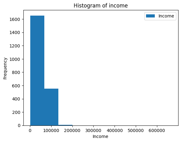
This doesn’t look very good because the x-axis extends so much!
- Looking at the data, can you figure out what might cause this?
When we look at the highest earners, we see that somebody put 666666 as their income.
We can assume that this was put as a joke or is an outlier.
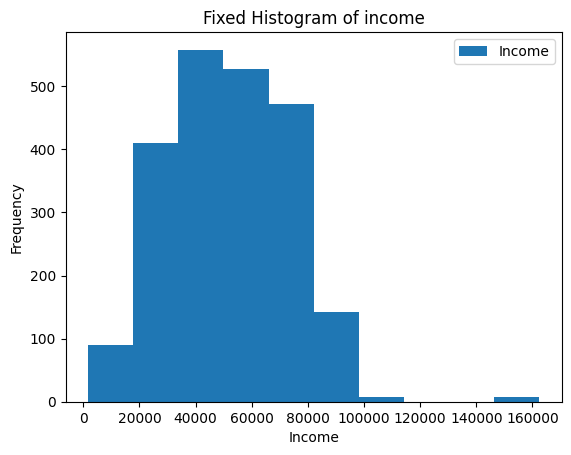
In either way, we can redo the plot with that datapoint removed.
- Can you “fix” the plot?
ax = merged_df[merged_df["Income"] != 666666].plot(kind="hist",y="Income")
ax.set_xlabel("Income")
ax.set_title("Fixed Histogram of income")
Text(0.5, 1.0, ‘Fixed Histogram of income’)
8.9.2 Bar plot
Another visualization we could do is a bar plot.
Using the groupby and mean methods, we can calculate the mean Income like we’ve learned before.
grouped_by_education = merged_df.groupby(by="Education")["Income"].mean()
grouped_by_education
Education
2n Cycle 47633.190000
Basic 20306.259259
Graduation 52720.373656
Master 52917.534247
PhD 56145.313929
Name: Income, dtype: float64Now, this data can be shown:
ax = grouped_by_education.plot(kind="bar")
ax.set_ylabel("Mean income")
ax.set_title("Mean income for each education level")
Text(0.5, 1.0, ‘Mean income for each education level’)

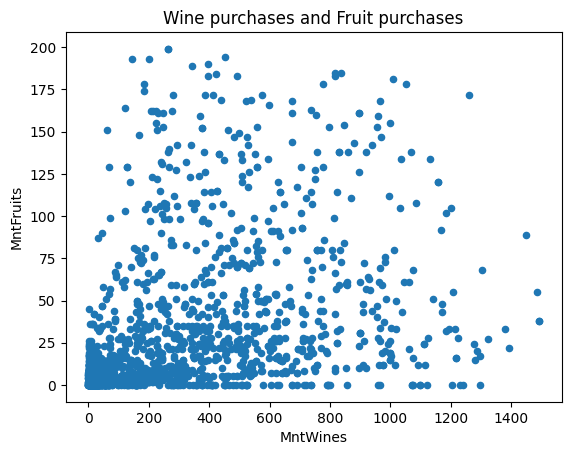
8.9.3 Scatter plot
Another kind of plot is the scatter plot, which needs two columns for the x and y axis.
ax = df.plot(kind="scatter", x="MntWines", y="MntFruits")
ax.set_title("Wine purchases and Fruit purchases")
Text(0.5, 1.0, ‘Wine purchases and Fruit purchases’)
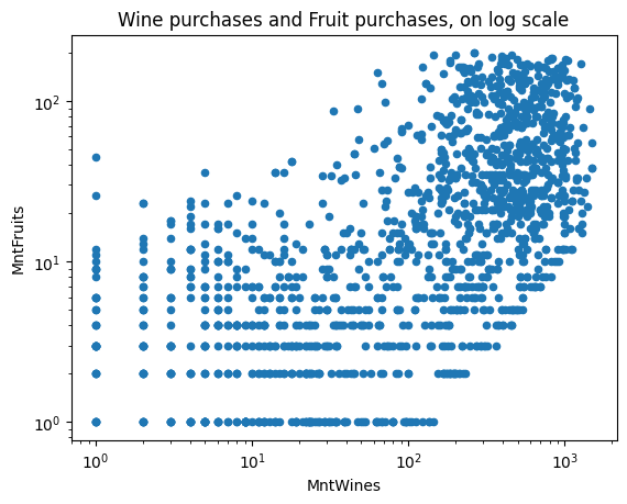
You can also specify whether the axes should be on the log scale or not.
ax = df.plot(kind="scatter", x="MntWines", y="MntFruits", logy=True, logx=True)
ax.set_title("Wine purchases and Fruit purchases, on log scale")
Text(0.5, 1.0, ‘Wine purchases and Fruit purchases, on log scale’)
8.10 Plotnine
Plotnine is the Python clone of ggplot2, which is very powerful and is great if you are already familiar with the ggplot2 syntax!
from plotnine import *(ggplot(merged_df, aes("Education", "MntWines", fill="Education"))
+ geom_boxplot(alpha=0.8))
(ggplot(merged_df[(merged_df["Year_Birth"]>1900) & (merged_df["Income"]!=666666)],
        aes("Year_Birth", "Income", fill="Education"))
 + geom_point(alpha=0.5, stroke=0)
 + facet_wrap("Marital_Status"))
task
Now that you are familiar with python, pandas, and plotting. There are two data.tables from AncientMetagenomeDir which contains metadata from metagenomes. You should, by using the code in the tutorial be able to explore the datasets and make some fancy plots.
file names:
sample_table_url
library_table_url
8.11 (Optional) clean-up
Let’s clean up your working directory by removing all the data and output from this chapter.
When closing your jupyter notebook(s), say no to saving any additional files.
Press ctrl + c on your terminal, and type y when requested. Once completed, the command below will remove the /<PATH>/<TO>/python-pandas directory as well as all of its contents.
Always be VERY careful when using rm -r. Check 3x that the path you are specifying is exactly what you want to delete and nothing more before pressing ENTER!
rm -r /<PATH>/<TO>/python-pandas*Once deleted you can move elsewhere (e.g. cd ~).
We can also get out of the conda environment with
conda deactivateTo delete the conda environment
conda remove --name python-pandas --all -y